

For more information click here for the Costing Climate Change to Public Infrastructure portal.
Glossary of Terms
Table of Abbreviations
Abbreviation Long Form
- AR5
- Fifth Assessment Report
- AR6
- Sixth Assessment Report
- CIPI
- Costing Climate Change Impact on Public Infrastructure (project)
- CRV
- Current Replacement Value
- IDF
- Intensity-Duration-Frequency (Curve)
- IPCC
- Intergovernmental Panel on Climate Change
- O&M
- Operation and Maintenance
- RCP
- Representative Concentration Pathway
- SME
- Subject-Matter Experts
- USL
- Useful Service Life
- WSP
- WSP Global Inc.
Definitions
Current Replacement Value: The current cost of rebuilding an asset with the equivalent capacity, functionality and performance.
Operations and Maintenance (O&M): The routine activities performed on an asset that maximize service life and minimize service disruptions.
Rehabilitation: Repairing part or most of an asset to extend its service life, without adding to its capacity, functionality or performance.
Renewal: Replacement of an existing asset, resulting in a new or as-new asset with an equivalent capacity, functionality and performance as the original asset. Renewal is different from rehabilitation, as renewal rebuilds the entire asset.
State of Good Repair: A performance standard which helps to maximize the benefits of public infrastructure in a cost-effective manner and ensures the assets operate in a condition that is considered acceptable from both an engineering and cost management perspective.
Stable Climate / Baseline Cost Projection: The operations and maintenance, rehabilitation, and renewal expense that would have been required to maintain public buildings in a state of good repair if climate indicators for extreme rainfall, extreme heat and freeze-thaw cycles remain unchanged from their 1975-2005 average levels over the projection to 2100.
Rest of the Century: Refers to the 79 years from 2022 to 2100.
Acute Hazard: Severe climate hazards that occur rarely (such as the 100-year storm event).
Chronic Hazard: Climate hazards that are changing gradually.
Retrofit: A retrofit is an adaptation made during the building’s service life.
Adaptation: Adaptation is modelled as an alteration of a building’s physical components to prevent more rapid deterioration and increased O&M expenses caused by changes in extreme rainfall and heat. Adaptation can be done through retrofit while an asset is still in service or can be done at the time of renewal.
No Adaptation Atrategy / Damage Costs: An asset management strategy where public buildings are not adapted to changing climate hazards. Under this strategy, additional costs are incurred from increased deterioration and higher O&M expenses caused by climate change hazards.
Reactive Adaptation Strategy: An asset management strategy where public buildings are only adapted at the time of renewal to withstand changing climate condition.
Proactive Adaptation Strategy: An asset management strategy where public buildings are adapted at the first available opportunity to withstand changing climate condition. This occurs either during a building’s next major rehabilitation through a retrofit or at renewal, whichever comes first.
1 | Introduction and context
In June 2019, a Member of Provincial Parliament asked the FAO to analyze the costs that climate change impacts could impose on Ontario’s provincial and municipal infrastructure, and how those costs could impact the long-term budget outlook of the province. In response to this request, the FAO launched its Costing Climate Change Impacts to Public Infrastructure project (CIPI).
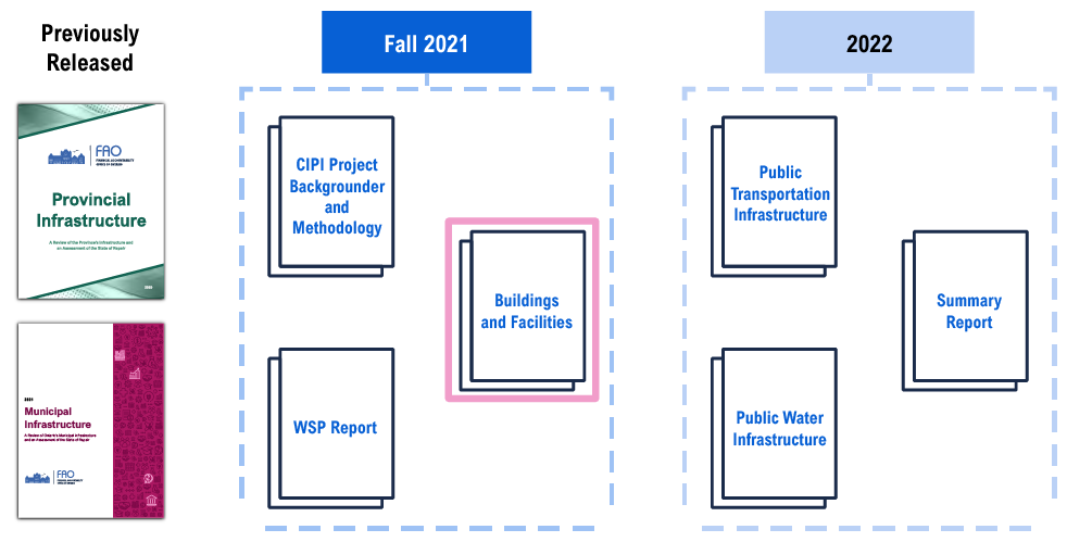
In the first two phases of the project, the FAO assessed the composition and state of repair of provincial and municipal infrastructure, with findings released in November 2020 and in August 2021. This report is the first of three sector reports that present the climate change costing results in the final phase of the project.
This report examines the impacts of changes in extreme rainfall, extreme heat and freeze-thaw cycles on the long-term costs of maintaining public buildings in a state of good repair. The project’s context, methodology and data sources are described in the FAO’s CIPI project backgrounder and methodology report.[1] Detailed information on the engineering aspects of the CIPI project can be found in WSP’s report.[2] Additional costing results and data downloads can be found on the FAO website.
2 | Summary
Ontario’s provincial and municipal governments own a large portfolio of public buildings and facilities
The FAO estimates that Ontario’s provincial and municipal governments currently own and manage about $254 billion[3] of public buildings and facilities. These assets include hospitals, schools, colleges, administration buildings, correctional facilities, courthouses, transit facilities, social housing, tourism, culture and sport facilities, as well as potable, storm water and wastewater facilities.
Keeping assets in a state of good repair helps to maximize the benefits of public infrastructure in the most cost-effective manner over time. This requires annual operations and maintenance (O&M) spending, as well as intermittent capital spending either to rehabilitate part(s) of an asset or to fully renew it at the end of its service life. The cost of maintaining Ontario’s portfolio of public buildings and facilities in a state of good repair would be around $10.1 billion[4] per year on average, totalling about $799 billion over the rest of the 21st century (2022-2100).[5] These projected “baseline costs” are what would have occurred in a stable climate.
Climate change will have a significant impact on the cost of maintaining public buildings in the absence of adaptation
To ensure safety and reliability, public infrastructure is designed, built and maintained to withstand a specific range of climate conditions typically based on historic climate data. However, extreme rainfall and extreme heat are projected to become more frequent and intense, while shorter winters will somewhat lower the annual number of freeze-thaw cycles. Taken together, the FAO estimates these hazards will add roughly $6 billion to the costs of maintaining public buildings and facilities in a state of good repair over the remainder of this decade (2022-2030).
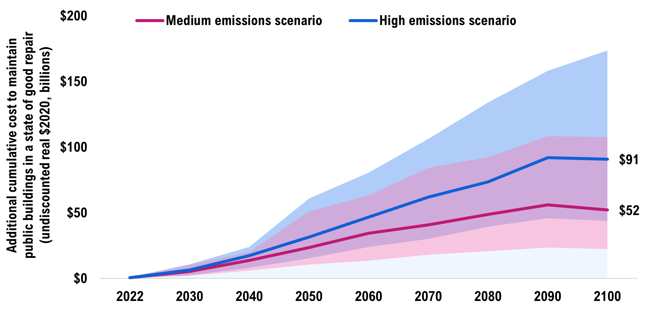
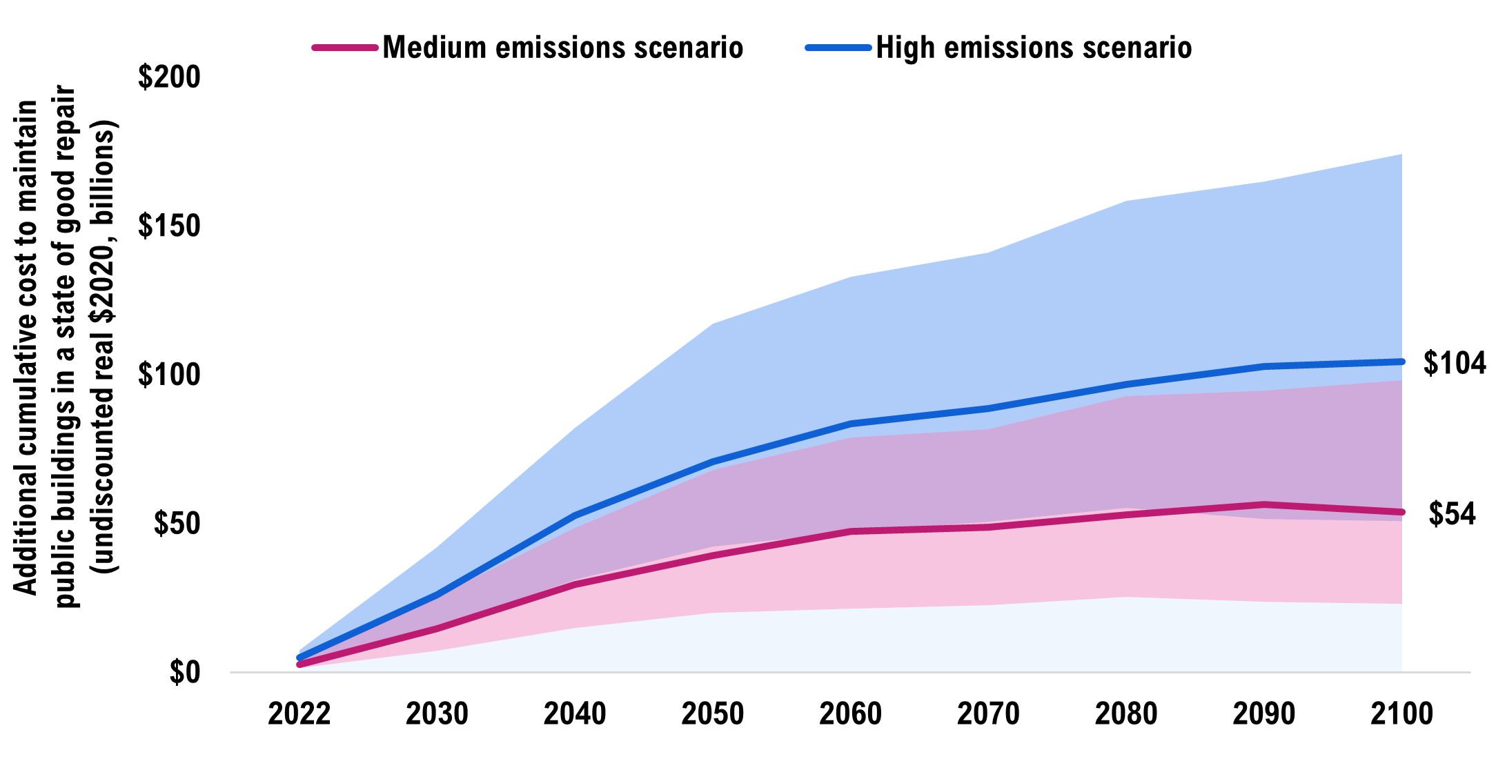
Over the long term, the extent of global climate change will influence the severity of these climate hazards and their impacts to public buildings. In a medium emissions scenario,[6] the cumulative cost of maintaining the existing portfolio of public buildings in a state of good repair will increase by $66 billion (8.2 per cent increase over baseline), or $0.8 billion per year on average over the rest of the 21st century. However, in a high emissions scenario,[7] cumulative costs would increase by $116 billion (14.5 per cent increase over baseline), or $1.5 billion per year on average over the rest of the century. These results reflect higher capital expenses from accelerated deterioration and higher O&M expenses.
Figure 2-1 More extreme rainfall and heat will raise the cost of maintaining the current portfolio of public buildings in the absence of adaptation actions
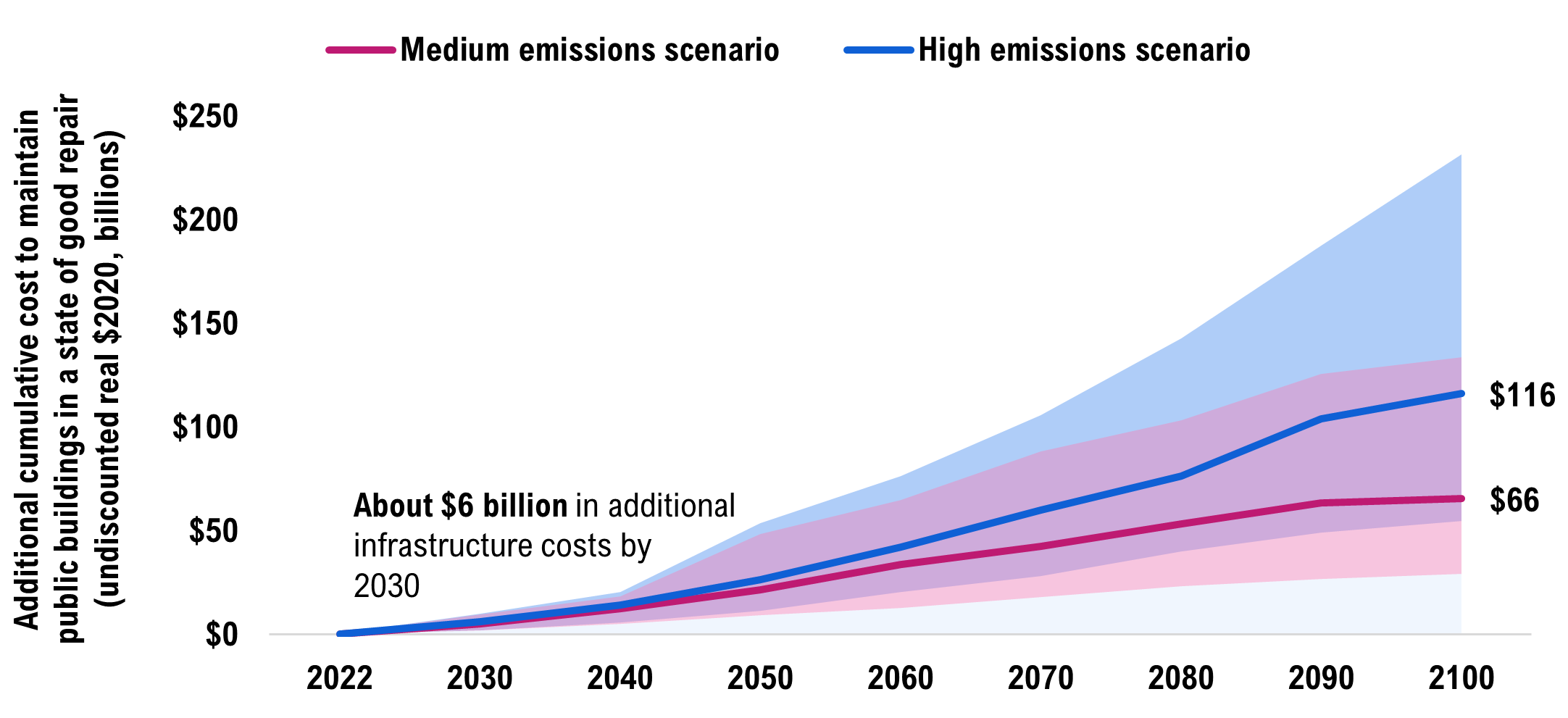
Notes: The solid line is the median (or 50th percentile) projection. The coloured bands represent the range of possible outcomes in each emissions scenario. The costs presented in this chart are in addition to the projected baseline costs over the same period.
Source: FAO.
Adapting public buildings to withstand these climate hazards will require significant investment
To explore the financial implications of adapting Ontario’s public buildings to withstand extreme rainfall and extreme heat,[8] the FAO costed two adaptation approaches: a reactive strategy and a proactive strategy.
The reactive strategy assumes public buildings are rebuilt to withstand late-century projections of extreme rainfall and extreme heat when they are replaced at the end of their service life, with 77 per cent of public buildings adapted by 2100.[9] Reactively adapting Ontario’s public buildings to withstand extreme rainfall and heat in the medium emissions scenario would cost an additional $52 billion (6.5 per cent over baseline) cumulatively to 2100, while adapting to climate conditions in the high emissions scenario would instead cost $91 billion (11.4 per cent over baseline).
The proactive strategy assumes most public buildings are retrofitted before the end of their service lives to withstand late-century projections of extreme rainfall and extreme heat, and nearly all assets are adapted by 2060. Proactively adapting this portfolio to withstand extreme rainfall and heat in the medium emissions scenario would cost an additional $54 billion (6.7 per cent over baseline) cumulatively to 2100, while adapting to climate conditions in the high emissions scenario would instead cost $104 billion (13.1 per cent over baseline).[10]
Adaptation will modestly lower the direct financial costs to provincial and municipal governments of maintaining public buildings over the long term
The financial impact of these climate hazards will be material to the province and municipalities regardless of which asset management strategy is pursued. However, this study only includes a narrow range of financial costs directly related to maintaining public buildings and facilities in a state of good repair. The societal costs of planned and unplanned service disruptions were beyond the scope of this report but would be significant.[11] These impacts would be much more significant for buildings that are not adapted.
Even within the narrow range of cost impacts analyzed in this report, the costs to governments in the adaptation strategies are modestly lower than the no adaptation strategy.[12] The comparative benefits of adaptation would be more significant if the indirect costs were incorporated.
Figure 2-2 The long-term cumulative costs of maintaining Ontario’s public buildings are modestly lower when adaptation actions are taken
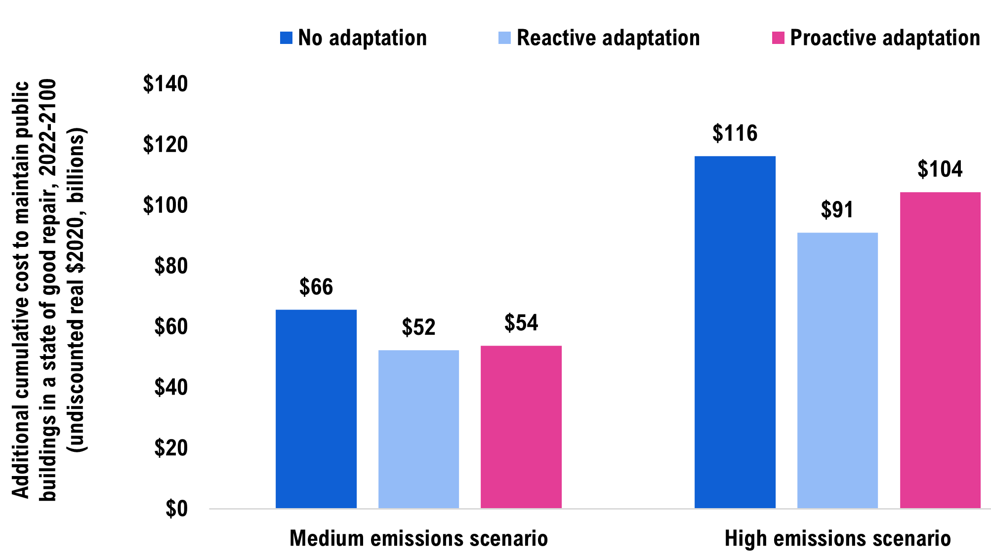
Notes: The costs presented in this chart are in addition to the baseline costs over the same period.
Source: FAO.
Determining the most cost-effective strategy for an individual asset would require comparing the costs of different adaptation strategies over its service life, for a broader range of climate hazards and societal costs, and with the asset’s specific circumstances taken into consideration. While the portfolio level costing results in this report are not intended to inform asset-specific management decisions, the results show that changes in extreme rainfall, extreme heat and freeze-thaw cycles will carry significant budgetary impacts for the province and Ontario’s municipalities.
3 | The long-term costs of maintaining public buildings
This chapter presents the scope of public buildings and facilities considered in this report, followed by a discussion of the costs necessary to maintain these assets in a state of good repair. Next, the chapter estimates the long-term infrastructure costs required to maintain Ontario’s buildings and facilities in a state of good repair to 2100 under a stable climate. The purpose of this chapter is to establish a baseline projection of infrastructure costs. In later chapters, this baseline is then be compared to projections that account for certain climate change hazards.
Ontario has a large portfolio of public buildings and facilities
This report focuses on buildings and facilities owned and controlled by provincial and municipal governments. The FAO estimates that the current replacement value[13] (CRV) of these assets is $254 billion in 2022, representing roughly 42 per cent of the total infrastructure examined within the CIPI project.[14]
Public buildings and facilities valued at $141 billion (55 per cent) are owned by the provincial government, while the remaining $113 billion (45 per cent) are owned by Ontario’s municipalities.[15] Provincial assets include:
- hospitals
- schools
- colleges
- government office buildings
- correctional facilities and courthouses
- transit facilities
Municipal assets include:
- social housing
- government administration buildings
- tourism buildings and facilities
- culture, recreation, and sport facilities
- potable water, storm water and wastewater management buildings and facilities
- transit facilities
Figure 3-1 Ontario’s portfolio of public buildings has a Current Replacement Value of $254 billion
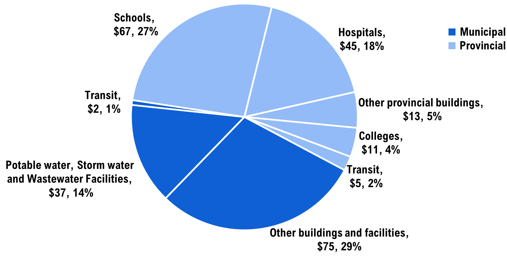
Note: CRV estimates are in real 2020 billion dollars. Percentage values refer to a sector’s share of total CRV.
Source: FAO.
Maintaining a large portfolio of buildings requires significant spending
Keeping assets in a state of good repair helps to maximize the benefits of public infrastructure in the most cost-effective manner over time. To be maintained in a state of good repair, assets require annual operations and maintenance (O&M) spending, as well as intermittent capital spending either to rehabilitate[16] an asset or renew it at the end of its service life.[17]
The age and condition of public buildings in Ontario’s portfolio vary significantly. To project the costs of maintaining public buildings in a state of good repair, the FAO gathered and estimated asset-specific information on age, condition and current replacement value, as well as the general performance standards used to evaluate if an asset is in a state of good repair. Using an infrastructure deterioration model based on modelling techniques developed by the Ontario Ministry of Infrastructure,[18] the FAO projected the capital and operating expenses necessary to maintain the current portfolio[19] of public buildings in a state of good repair to 2100.
These long-term O&M, rehabilitation and renewal spending estimates form the baseline projection against which the climate change costing scenarios developed in later chapters will be compared. The baseline projection represents the infrastructure costs that would have been required to maintain public buildings in a stable climate.[20]
While O&M expenses occur annually, the timing of rehabilitation and renewal expenses depends on a building’s age and condition. Figure 3-2 shows the annual proportion of Ontario’s public buildings (by CRV) that would require rehabilitation or renewal spending over the rest of this century if the funding necessary to bring and maintain the current portfolio of public buildings into a state of good repair were made available and spent in a timely manner.[21] On average, around six per cent of buildings will require rehabilitation or renewal every year.
Figure 3-2 Proportion of public buildings requiring rehabilitation or renewal each year
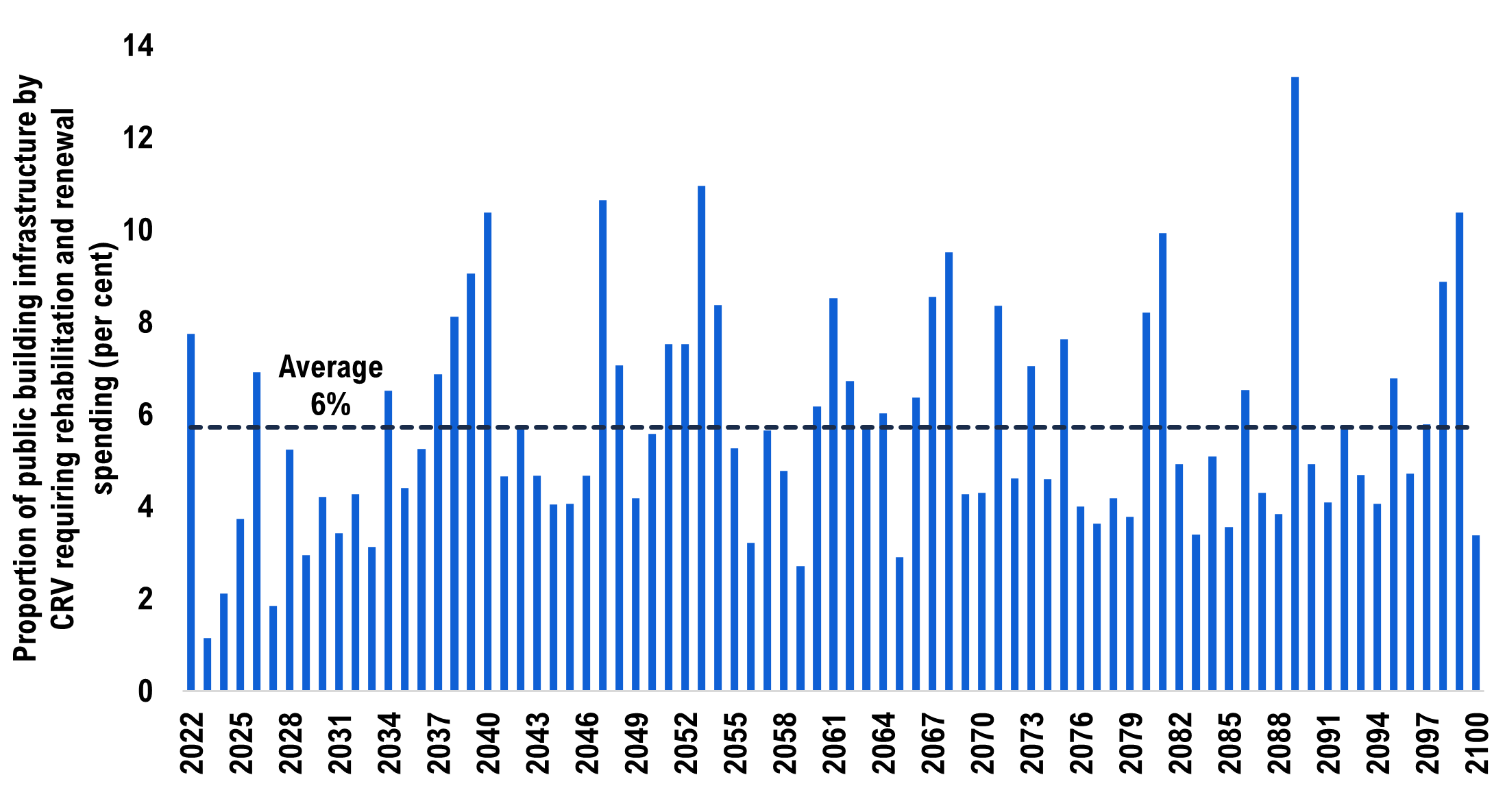
Source: FAO.
$799 billion needed to maintain public buildings until 2100 in a stable climate
Bringing Ontario’s existing suite of public buildings into a state of good repair and maintaining them until 2100 would cost $799 billion cumulatively in a stable climate, or an average of about $10 billion per year. This baseline cost includes $296 billion in cumulative O&M expense and $503 billion in rehabilitation and renewal expense to 2100.
The costs to maintain public buildings in a state of good repair reflect both the value of assets owned, as well as the condition, age and performance standards of each individual asset under management. For example, assets in poorer condition require more capital spending to bring them into a state of good repair. Likewise, older assets must be renewed sooner than newer assets.
Figure 3-3 The cumulative cost of maintaining Ontario’s public buildings and facilities in a state of good repair to 2100 in a stable climate
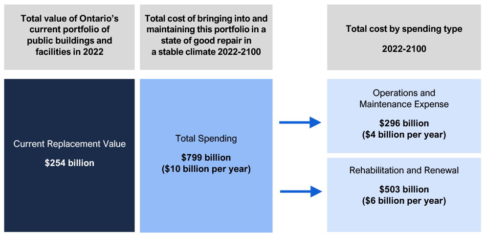
Note: All values presented in real 2020 dollars.
Source: FAO.
Accessible version
In a stable climate, the cumulative cost of bringing and maintaining Ontario’s existing suite of public buildings into a state of good repair until 2100 would be $799 billion, or an average of roughly $10 billion per year. This baseline cost includes $296 billion in cumulative O&M expense and $503 billion in rehabilitation and renewal expense to 2100.
4 | The cost of key climate hazards to public buildings
Climate change is associated with many hazards to public infrastructure, which can take the form of extreme weather events or long-term chronic impacts, that affect asset deterioration. Ontario has been subject to costly floods and ice storms and is also prone to droughts, intense rainfall, wildfires, windstorms, heatwaves and permafrost melt.[22] This project focuses on only three climate hazards – extreme rainfall, extreme heat and freeze-thaw cycles – as they were determined to have broad and financially material impacts to public infrastructure and can be projected with a reasonable degree of scientific confidence.[23]
This chapter summarizes how projected changes in these climate hazards would impact Ontario’s public buildings in the absence of adaptation measures. It then presents the FAO’s estimates of the additional long-term costs these climate hazards would impose on Ontario’s portfolio of public buildings in medium and high emissions scenarios.
Extreme rainfall, extreme heat and freeze-thaw cycles
To ensure safety and reliability, infrastructure is designed, built and maintained to withstand a specific range of climate conditions typically based on historic climatic loads.[24] However, extreme rainfall and extreme heat are projected to increase in the future, while freeze-thaw cycles are projected to decrease.
Extreme rainfall can often exceed the capacity of infrastructure drainage systems and lead to flooding, water infiltration or increased erosion of infrastructure components.[25] Extreme rainfall events can impact buildings as acute hazards that occur rarely (for example the 100-year rainfall event).[26] Extreme rainfall can also cause chronic impacts, such as ongoing moisture or water infiltration. This hazard includes the impacts of pluvial flooding (i.e., overwhelmed drainage systems) but not the impacts of fluvial flooding (i.e., riverine or river flooding).
Extreme heat events are extended spells of high temperatures. As heatwaves increase in frequency and duration, temperatures will more frequently exceed the capacity of infrastructure or its components, increase the stress on building materials, and impact operations and maintenance. Extreme temperatures are both a chronic and an acute hazard. For example, thermal expansion in brick walls during a high-magnitude heat wave is an acute impact, while the accelerated deterioration of air conditioning equipment used more frequently in warmer conditions is a chronic impact.
Freeze-thaw cycles (FTCs) are fluctuations between freezing and non-freezing temperatures that cause water to freeze (and expand) or melt (and contract). The melting and re-freezing of water accelerates the weathering of building materials, and damages infrastructure components that are exposed to the atmosphere. FTC damage is caused by the combination of temperature fluctuations around zero degrees and the presence of water.[27] FTCs can be self reinforcing. When one occurs, it can leave cracks or gaps in building materials, creating the potential for further water infiltration and another cycle of freezing and expansion. “Deep” FTCs typically occur in winter and are defined as those that occur when the daily average temperature is less than 0°C.
Changes in these three climate hazards will impact Ontario’s public buildings and facilities in different ways. A typical building has many components, including its structure, envelope, equipment and finishing, mechanical and electrical systems, as well as civil infrastructure and landscaping. Figure 3‑1 describes these key building components and provides examples of the interaction between those components and the three climate hazards.
Figure 4-1 Examples of climate hazard impacts to key components of public building infrastructure
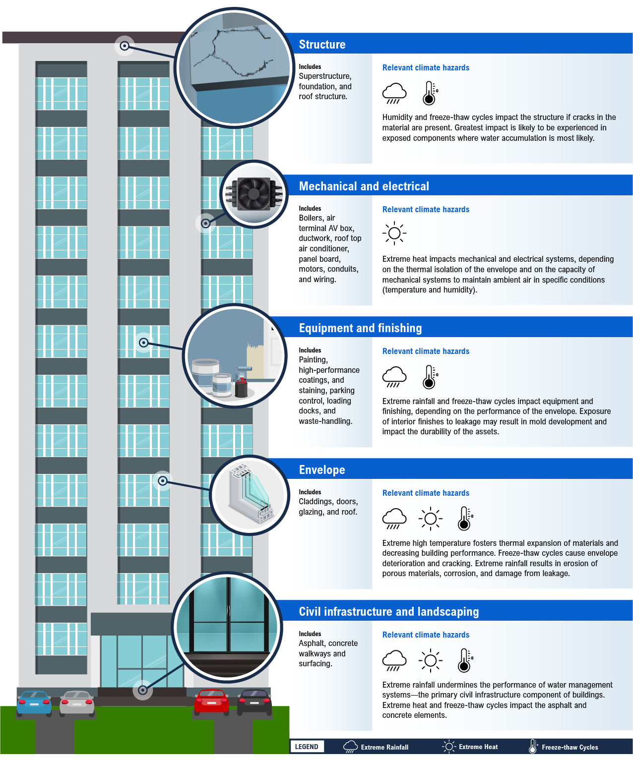
Note: For more examples of how these climate hazards impact building components, see WSP 2021.
Source: WSP.
Most climate hazards to public buildings will increase
The impacts of changing climate hazards on Ontario’s public buildings depend on the path of global greenhouse gas emissions and the extent of global mean temperature increases. The FAO costed climate impacts to public buildings for three global emissions scenarios:
- A low emissions scenario that assumes a major and immediate turnaround in global climate policies. Emissions are projected to peak in the early 2020s and decline to zero by the 2080s. By the end of the century, net emissions are negative. In this scenario, global mean temperatures are projected to increase by 1.6°C (0.8 to 2.4°C) by 2100 compared to the pre-industrial average (1850-1900).[28] The key results for this scenario are presented in Appendix E.
- A medium emissions scenario, where global emissions peak in the 2040s, then decline rapidly over the following four decades before stabilizing at the end of the century. In this scenario, the global mean temperature is projected to increase by 2.3°C (1.7 to 3.2°C) by 2100 relative to 1850-1900.
- A high emissions scenario that assumes global emissions continue to grow for most of the century.[29] Global mean temperatures are projected to increase by 4.2°C (3.2 to 5.4°C) relative to 1850-1900. Cumulative emissions from 2005 to 2020 most closely match the high emissions scenario.[30]
Uncertainty in climate change projections
The FAO partnered with the Canadian Centre for Climate Services at Environment Canada to acquire projections of key climate indicators for Ontario. To account for uncertainty in climate projections and in line with common practice in climate science, the median (50th percentile) projections of climate variables are presented, followed by ranges in parentheses. For Ontario climate indicators, the ranges indicate the 10th and 90th percentile projections from the ensemble of 24 climate models used by the Canadian Centre for Climate Services.
Figure 4-2 presents a brief description of the projected changes in some of the climate indicators used to represent these hazards. Appendix B contains a full description of all relevant climate variables to public buildings, and their trends in all scenarios
Figure 4-2 Changing climate hazards in Ontario
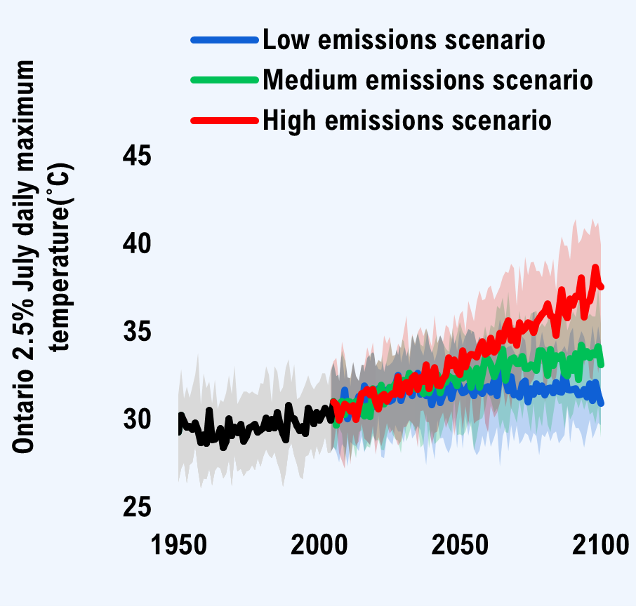
- Projected changes in Ontario’s peak July temperatures differ significantly in the low and high emissions scenarios. Compared to the 1976-2005 average, the base period for this report, Ontario’s peak July temperatures are projected to be 1.7°C (1.3 to 2.0°C) higher in the low emissions scenario by the 2030s. By the 2080s, peak July temperatures are projected to increase by 1.9°C (0.9 to 2.8°C) in the low emissions scenario and by 6.5°C (4.3 to 7.6°C) in the high emissions scenario.
- There is high confidence in the projected trends and ranges of temperature variables based on strong scientific evidence in the causes of observed changes.
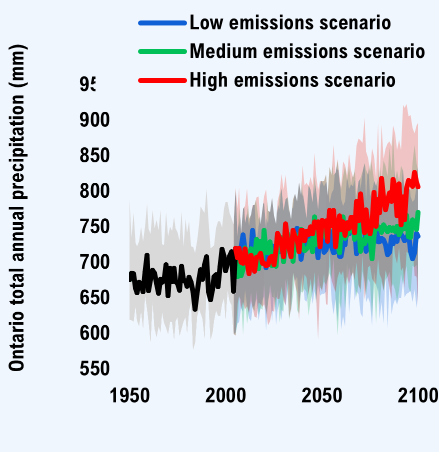
- Average annual precipitation in Ontario is projected to increase by 6.0 per cent (5.3 to 6.6 per cent) in the low emissions scenario by the 2030s. By the 2080s, average annual precipitation is projected to rise by 7.1 per cent (4.0 to 7.8 per cent) in the low emissions scenario and by 15.0 per cent (6.2 to 18.2 per cent) in the high emissions scenario.
- Confidence in the projected trends and ranges of aggregate precipitation variables is somewhat lower (high-to-medium) than for temperature variables as there is less confidence in how well climate models represent the climate processes involved.
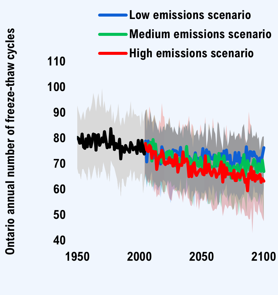
- Annual FTCs are the number of days in a year when the temperature crosses 0°C. Over the coming decades, the winter season will shorten due to rising temperatures. Ontario average FTCs are projected to decline by 4.9 per cent (1.5 to 11.9 per cent) in the low emissions scenario by the 2030s. By the 2080s, annual FTCs are projected to decrease by 5.5 per cent (0 to 15.2 per cent) in the low emissions scenario and by 15.1 per cent (0 to 24.9 per cent) in the high emissions scenario.
- There is high confidence in the projections of annual FTCs and medium confidence in deep FTCs based on the amount of evidence for projected trends and ranges.
Source: Canadian Centre for Climate Services.
Accessible version
| Low Emissions Scenario | Medium-Emissions Scenario | High-Emissions Scenario | |||||||
|---|---|---|---|---|---|---|---|---|---|
| Year | Low | Median | High | Low | Median | High | Low | Median | High |
| 1950 | 619 | 676 | 787 | 619 | 676 | 787 | 619 | 676 | 788 |
| 1951 | 618 | 684 | 734 | 618 | 684 | 734 | 618 | 684 | 734 |
| 1952 | 618 | 684 | 771 | 617 | 684 | 770 | 616 | 684 | 771 |
| 1953 | 639 | 663 | 727 | 639 | 663 | 727 | 639 | 663 | 727 |
| 1954 | 618 | 657 | 722 | 619 | 657 | 722 | 619 | 657 | 722 |
| 1955 | 610 | 672 | 730 | 611 | 672 | 730 | 611 | 672 | 730 |
| 1956 | 632 | 670 | 750 | 632 | 670 | 750 | 632 | 669 | 750 |
| 1957 | 606 | 659 | 730 | 609 | 659 | 730 | 607 | 659 | 730 |
| 1958 | 654 | 686 | 750 | 654 | 685 | 749 | 654 | 686 | 750 |
| 1959 | 635 | 709 | 782 | 635 | 709 | 782 | 635 | 710 | 782 |
| 1960 | 617 | 659 | 747 | 617 | 659 | 747 | 617 | 660 | 747 |
| 1961 | 588 | 676 | 740 | 588 | 676 | 740 | 588 | 676 | 740 |
| 1962 | 646 | 688 | 773 | 646 | 688 | 775 | 646 | 688 | 773 |
| 1963 | 607 | 684 | 749 | 607 | 684 | 748 | 607 | 684 | 748 |
| 1964 | 594 | 667 | 760 | 595 | 669 | 760 | 596 | 671 | 760 |
| 1965 | 610 | 657 | 745 | 610 | 656 | 745 | 610 | 657 | 745 |
| 1966 | 605 | 676 | 774 | 601 | 676 | 774 | 604 | 676 | 774 |
| 1967 | 630 | 670 | 726 | 630 | 672 | 726 | 630 | 672 | 725 |
| 1968 | 615 | 675 | 722 | 616 | 674 | 723 | 615 | 674 | 725 |
| 1969 | 608 | 697 | 770 | 608 | 697 | 770 | 608 | 697 | 770 |
| 1970 | 599 | 653 | 736 | 599 | 654 | 736 | 601 | 653 | 736 |
| 1971 | 616 | 692 | 750 | 616 | 692 | 750 | 616 | 692 | 750 |
| 1972 | 618 | 674 | 744 | 617 | 673 | 744 | 616 | 673 | 744 |
| 1973 | 592 | 692 | 764 | 592 | 692 | 763 | 592 | 692 | 764 |
| 1974 | 618 | 674 | 748 | 617 | 673 | 747 | 617 | 673 | 748 |
| 1975 | 623 | 670 | 744 | 624 | 670 | 743 | 623 | 670 | 742 |
| 1976 | 596 | 661 | 730 | 596 | 661 | 730 | 596 | 661 | 730 |
| 1977 | 607 | 694 | 771 | 607 | 694 | 771 | 607 | 694 | 771 |
| 1978 | 617 | 673 | 722 | 617 | 673 | 722 | 617 | 674 | 722 |
| 1979 | 625 | 674 | 761 | 622 | 674 | 761 | 622 | 674 | 761 |
| 1980 | 600 | 667 | 743 | 602 | 667 | 741 | 601 | 666 | 741 |
| 1981 | 633 | 679 | 758 | 632 | 679 | 758 | 632 | 679 | 758 |
| 1982 | 643 | 671 | 723 | 643 | 672 | 722 | 644 | 672 | 723 |
| 1983 | 576 | 658 | 724 | 577 | 658 | 723 | 577 | 659 | 722 |
| 1984 | 587 | 635 | 711 | 587 | 635 | 711 | 586 | 634 | 713 |
| 1985 | 623 | 656 | 730 | 624 | 656 | 731 | 624 | 656 | 730 |
| 1986 | 635 | 679 | 753 | 635 | 678 | 753 | 635 | 677 | 753 |
| 1987 | 628 | 689 | 779 | 629 | 690 | 780 | 629 | 689 | 778 |
| 1988 | 622 | 676 | 772 | 620 | 676 | 774 | 621 | 676 | 773 |
| 1989 | 592 | 698 | 769 | 594 | 697 | 769 | 593 | 696 | 769 |
| 1990 | 668 | 707 | 802 | 668 | 708 | 802 | 667 | 708 | 803 |
| 1991 | 642 | 659 | 757 | 641 | 659 | 759 | 642 | 658 | 758 |
| 1992 | 591 | 648 | 719 | 591 | 648 | 719 | 590 | 647 | 720 |
| 1993 | 602 | 663 | 720 | 602 | 661 | 721 | 601 | 662 | 722 |
| 1994 | 619 | 677 | 725 | 619 | 680 | 724 | 619 | 680 | 724 |
| 1995 | 632 | 680 | 748 | 633 | 681 | 748 | 632 | 682 | 748 |
| 1996 | 628 | 665 | 757 | 627 | 665 | 758 | 625 | 666 | 757 |
| 1997 | 624 | 693 | 757 | 624 | 694 | 757 | 624 | 694 | 758 |
| 1998 | 642 | 718 | 749 | 643 | 717 | 751 | 641 | 718 | 749 |
| 1999 | 650 | 709 | 776 | 651 | 709 | 776 | 650 | 708 | 776 |
| 2000 | 620 | 691 | 783 | 619 | 690 | 787 | 620 | 688 | 785 |
| 2001 | 661 | 697 | 786 | 662 | 697 | 786 | 660 | 698 | 785 |
| 2002 | 645 | 708 | 769 | 647 | 708 | 770 | 646 | 708 | 769 |
| 2003 | 639 | 715 | 761 | 640 | 715 | 761 | 640 | 715 | 762 |
| 2004 | 599 | 658 | 756 | 600 | 659 | 753 | 599 | 659 | 753 |
| 2005 | 601 | 719 | 804 | 597 | 719 | 804 | 597 | 719 | 805 |
| 2006 | 614 | 684 | 758 | 618 | 680 | 736 | 641 | 706 | 776 |
| 2007 | 616 | 685 | 748 | 652 | 717 | 776 | 653 | 719 | 805 |
| 2008 | 636 | 721 | 778 | 647 | 681 | 752 | 635 | 700 | 742 |
| 2009 | 630 | 738 | 805 | 597 | 690 | 809 | 644 | 698 | 775 |
| 2010 | 660 | 716 | 757 | 648 | 721 | 756 | 634 | 719 | 780 |
| 2011 | 640 | 711 | 769 | 613 | 697 | 769 | 638 | 701 | 804 |
| 2012 | 621 | 685 | 751 | 633 | 711 | 788 | 629 | 684 | 761 |
| 2013 | 617 | 715 | 769 | 657 | 719 | 803 | 645 | 710 | 767 |
| 2014 | 637 | 745 | 800 | 636 | 708 | 774 | 637 | 701 | 780 |
| 2015 | 639 | 719 | 783 | 631 | 704 | 801 | 623 | 687 | 781 |
| 2016 | 649 | 694 | 726 | 660 | 732 | 781 | 622 | 707 | 791 |
| 2017 | 617 | 708 | 752 | 626 | 691 | 761 | 644 | 707 | 793 |
| 2018 | 636 | 698 | 767 | 635 | 729 | 766 | 641 | 713 | 753 |
| 2019 | 647 | 711 | 775 | 633 | 703 | 781 | 638 | 699 | 776 |
| 2020 | 652 | 716 | 797 | 669 | 745 | 783 | 641 | 699 | 793 |
| 2021 | 604 | 692 | 763 | 627 | 713 | 748 | 632 | 695 | 803 |
| 2022 | 647 | 702 | 754 | 642 | 714 | 823 | 611 | 697 | 772 |
| 2023 | 659 | 722 | 792 | 668 | 729 | 785 | 617 | 706 | 771 |
| 2024 | 616 | 723 | 794 | 652 | 695 | 795 | 632 | 708 | 791 |
| 2025 | 660 | 697 | 776 | 650 | 713 | 800 | 631 | 697 | 765 |
| 2026 | 612 | 713 | 808 | 630 | 695 | 803 | 651 | 718 | 754 |
| 2027 | 632 | 723 | 786 | 660 | 721 | 770 | 648 | 741 | 786 |
| 2028 | 644 | 715 | 775 | 615 | 732 | 793 | 649 | 734 | 798 |
| 2029 | 618 | 720 | 808 | 633 | 734 | 804 | 666 | 725 | 824 |
| 2030 | 653 | 708 | 772 | 630 | 700 | 773 | 646 | 708 | 802 |
| 2031 | 638 | 736 | 810 | 676 | 724 | 789 | 639 | 754 | 823 |
| 2032 | 657 | 738 | 787 | 658 | 740 | 792 | 677 | 732 | 794 |
| 2033 | 670 | 720 | 771 | 619 | 721 | 791 | 622 | 720 | 776 |
| 2034 | 629 | 715 | 780 | 634 | 736 | 785 | 634 | 708 | 761 |
| 2035 | 685 | 723 | 776 | 652 | 702 | 799 | 685 | 745 | 789 |
| 2036 | 674 | 740 | 802 | 683 | 740 | 806 | 668 | 736 | 797 |
| 2037 | 679 | 748 | 813 | 633 | 718 | 839 | 658 | 733 | 785 |
| 2038 | 644 | 737 | 812 | 628 | 729 | 835 | 618 | 715 | 812 |
| 2039 | 662 | 704 | 803 | 659 | 747 | 829 | 678 | 745 | 795 |
| 2040 | 684 | 719 | 793 | 657 | 720 | 800 | 657 | 745 | 837 |
| 2041 | 647 | 725 | 804 | 662 | 716 | 782 | 683 | 730 | 808 |
| 2042 | 645 | 738 | 809 | 658 | 719 | 761 | 678 | 744 | 812 |
| 2043 | 659 | 735 | 806 | 625 | 723 | 809 | 653 | 739 | 808 |
| 2044 | 669 | 740 | 815 | 645 | 731 | 802 | 677 | 750 | 820 |
| 2045 | 641 | 741 | 833 | 657 | 715 | 784 | 657 | 740 | 808 |
| 2046 | 660 | 728 | 796 | 674 | 764 | 821 | 686 | 757 | 854 |
| 2047 | 647 | 730 | 818 | 642 | 725 | 802 | 653 | 749 | 824 |
| 2048 | 668 | 706 | 798 | 684 | 726 | 774 | 591 | 757 | 802 |
| 2049 | 653 | 745 | 818 | 664 | 747 | 808 | 667 | 722 | 815 |
| 2050 | 656 | 736 | 813 | 662 | 747 | 821 | 659 | 759 | 814 |
| 2051 | 656 | 714 | 807 | 673 | 749 | 814 | 684 | 757 | 814 |
| 2052 | 658 | 718 | 812 | 668 | 735 | 862 | 641 | 758 | 823 |
| 2053 | 675 | 727 | 812 | 675 | 740 | 842 | 640 | 730 | 793 |
| 2054 | 694 | 744 | 783 | 685 | 759 | 898 | 718 | 773 | 834 |
| 2055 | 647 | 722 | 797 | 676 | 769 | 845 | 674 | 751 | 823 |
| 2056 | 626 | 713 | 803 | 706 | 757 | 822 | 665 | 773 | 866 |
| 2057 | 649 | 715 | 839 | 646 | 726 | 826 | 657 | 721 | 824 |
| 2058 | 617 | 745 | 830 | 597 | 725 | 843 | 678 | 750 | 845 |
| 2059 | 670 | 708 | 831 | 644 | 713 | 813 | 687 | 765 | 821 |
| 2060 | 605 | 708 | 789 | 634 | 746 | 803 | 681 | 746 | 806 |
| 2061 | 624 | 724 | 779 | 679 | 764 | 821 | 688 | 757 | 842 |
| 2062 | 610 | 724 | 785 | 633 | 734 | 835 | 667 | 738 | 837 |
| 2063 | 698 | 755 | 820 | 667 | 738 | 815 | 680 | 756 | 822 |
| 2064 | 628 | 740 | 803 | 693 | 744 | 835 | 669 | 748 | 854 |
| 2065 | 661 | 746 | 810 | 680 | 745 | 810 | 681 | 763 | 829 |
| 2066 | 696 | 744 | 806 | 686 | 756 | 827 | 686 | 762 | 820 |
| 2067 | 646 | 751 | 817 | 668 | 732 | 835 | 674 | 742 | 828 |
| 2068 | 659 | 712 | 769 | 651 | 760 | 794 | 700 | 785 | 864 |
| 2069 | 655 | 732 | 832 | 670 | 753 | 814 | 667 | 758 | 874 |
| 2070 | 628 | 757 | 803 | 656 | 715 | 819 | 662 | 796 | 871 |
| 2071 | 622 | 759 | 826 | 688 | 732 | 828 | 709 | 767 | 868 |
| 2072 | 682 | 747 | 840 | 672 | 726 | 840 | 648 | 742 | 903 |
| 2073 | 644 | 715 | 787 | 654 | 731 | 830 | 663 | 774 | 856 |
| 2074 | 650 | 748 | 843 | 677 | 754 | 824 | 693 | 751 | 847 |
| 2075 | 643 | 718 | 793 | 671 | 735 | 851 | 695 | 740 | 828 |
| 2076 | 610 | 716 | 800 | 623 | 705 | 836 | 676 | 755 | 860 |
| 2077 | 687 | 750 | 813 | 670 | 738 | 815 | 673 | 798 | 849 |
| 2078 | 668 | 756 | 826 | 613 | 756 | 807 | 668 | 750 | 818 |
| 2079 | 659 | 728 | 786 | 665 | 747 | 819 | 704 | 788 | 896 |
| 2080 | 619 | 729 | 797 | 639 | 749 | 840 | 683 | 769 | 813 |
| 2081 | 643 | 734 | 806 | 673 | 742 | 815 | 677 | 818 | 894 |
| 2082 | 613 | 731 | 808 | 659 | 752 | 843 | 660 | 792 | 846 |
| 2083 | 687 | 725 | 785 | 676 | 748 | 835 | 689 | 774 | 860 |
| 2084 | 606 | 711 | 796 | 680 | 743 | 821 | 679 | 787 | 867 |
| 2085 | 674 | 714 | 802 | 686 | 749 | 863 | 663 | 798 | 870 |
| 2086 | 626 | 736 | 787 | 666 | 745 | 828 | 648 | 786 | 863 |
| 2087 | 639 | 726 | 806 | 669 | 748 | 882 | 733 | 817 | 893 |
| 2088 | 648 | 735 | 832 | 661 | 744 | 815 | 709 | 805 | 882 |
| 2089 | 640 | 730 | 775 | 645 | 751 | 829 | 698 | 765 | 858 |
| 2090 | 650 | 749 | 803 | 660 | 738 | 814 | 721 | 810 | 872 |
| 2091 | 649 | 740 | 798 | 684 | 744 | 835 | 688 | 753 | 858 |
| 2092 | 674 | 735 | 835 | 669 | 748 | 829 | 693 | 792 | 921 |
| 2093 | 651 | 730 | 787 | 683 | 747 | 802 | 662 | 760 | 917 |
| 2094 | 656 | 733 | 847 | 695 | 766 | 808 | 714 | 804 | 923 |
| 2095 | 657 | 741 | 825 | 664 | 736 | 805 | 712 | 815 | 905 |
| 2096 | 660 | 715 | 793 | 657 | 735 | 801 | 701 | 812 | 907 |
| 2097 | 643 | 705 | 785 | 695 | 760 | 840 | 725 | 807 | 889 |
| 2098 | 662 | 713 | 789 | 693 | 754 | 865 | 681 | 826 | 881 |
| 2099 | 635 | 740 | 807 | 696 | 746 | 839 | 680 | 812 | 893 |
| 2100 | 659 | 736 | 847 | 671 | 771 | 829 | 638 | 806 | 896 |
| Low Emissions Scenario | Medium-Emissions Scenario | High-Emissions Scenario | |||||||
|---|---|---|---|---|---|---|---|---|---|
| Year | Low | Median | High | Low | Median | High | Low | Median | High |
| 1950 | 26 | 29 | 31 | 26 | 29 | 31 | 26 | 29 | 31 |
| 1951 | 27 | 30 | 33 | 27 | 30 | 33 | 27 | 30 | 33 |
| 1952 | 28 | 30 | 31 | 28 | 30 | 31 | 28 | 30 | 31 |
| 1953 | 26 | 30 | 32 | 26 | 30 | 32 | 26 | 30 | 32 |
| 1954 | 27 | 30 | 31 | 27 | 30 | 31 | 27 | 30 | 31 |
| 1955 | 28 | 29 | 32 | 28 | 29 | 32 | 28 | 29 | 32 |
| 1956 | 29 | 30 | 33 | 29 | 30 | 33 | 29 | 30 | 33 |
| 1957 | 27 | 29 | 34 | 27 | 29 | 34 | 27 | 29 | 34 |
| 1958 | 26 | 29 | 31 | 26 | 29 | 31 | 26 | 29 | 31 |
| 1959 | 27 | 29 | 33 | 27 | 29 | 33 | 27 | 29 | 33 |
| 1960 | 27 | 29 | 32 | 27 | 29 | 32 | 27 | 29 | 32 |
| 1961 | 27 | 31 | 32 | 27 | 31 | 32 | 27 | 31 | 32 |
| 1962 | 26 | 29 | 31 | 26 | 29 | 31 | 26 | 29 | 31 |
| 1963 | 27 | 29 | 32 | 27 | 29 | 32 | 27 | 29 | 32 |
| 1964 | 27 | 29 | 31 | 27 | 29 | 31 | 27 | 29 | 31 |
| 1965 | 27 | 29 | 31 | 27 | 29 | 31 | 27 | 29 | 31 |
| 1966 | 27 | 28 | 31 | 27 | 28 | 31 | 27 | 28 | 31 |
| 1967 | 27 | 29 | 32 | 27 | 29 | 32 | 27 | 29 | 32 |
| 1968 | 28 | 30 | 33 | 28 | 30 | 33 | 28 | 30 | 33 |
| 1969 | 26 | 29 | 31 | 26 | 29 | 31 | 26 | 29 | 31 |
| 1970 | 28 | 30 | 33 | 28 | 30 | 33 | 28 | 30 | 33 |
| 1971 | 27 | 29 | 31 | 27 | 29 | 31 | 27 | 29 | 31 |
| 1972 | 27 | 30 | 31 | 27 | 30 | 31 | 27 | 30 | 31 |
| 1973 | 27 | 29 | 32 | 27 | 29 | 32 | 27 | 29 | 32 |
| 1974 | 27 | 29 | 32 | 27 | 29 | 32 | 27 | 29 | 32 |
| 1975 | 27 | 30 | 31 | 27 | 30 | 31 | 27 | 30 | 31 |
| 1976 | 27 | 30 | 32 | 27 | 30 | 32 | 27 | 30 | 32 |
| 1977 | 27 | 30 | 31 | 27 | 30 | 31 | 27 | 30 | 31 |
| 1978 | 28 | 29 | 31 | 28 | 29 | 31 | 28 | 29 | 31 |
| 1979 | 27 | 29 | 32 | 27 | 29 | 32 | 27 | 29 | 32 |
| 1980 | 28 | 30 | 32 | 28 | 30 | 32 | 28 | 30 | 32 |
| 1981 | 28 | 30 | 33 | 28 | 30 | 33 | 28 | 30 | 33 |
| 1982 | 28 | 29 | 32 | 28 | 29 | 33 | 28 | 29 | 33 |
| 1983 | 28 | 30 | 31 | 28 | 30 | 31 | 28 | 30 | 31 |
| 1984 | 28 | 30 | 33 | 28 | 30 | 33 | 28 | 30 | 33 |
| 1985 | 28 | 30 | 33 | 28 | 30 | 33 | 28 | 30 | 33 |
| 1986 | 27 | 30 | 31 | 27 | 30 | 32 | 27 | 30 | 32 |
| 1987 | 26 | 29 | 32 | 26 | 29 | 32 | 26 | 29 | 32 |
| 1988 | 27 | 29 | 33 | 27 | 29 | 33 | 27 | 29 | 33 |
| 1989 | 28 | 31 | 33 | 28 | 31 | 33 | 28 | 31 | 33 |
| 1990 | 29 | 30 | 32 | 29 | 30 | 32 | 29 | 30 | 32 |
| 1991 | 28 | 30 | 33 | 28 | 30 | 33 | 28 | 30 | 33 |
| 1992 | 27 | 30 | 31 | 27 | 30 | 31 | 27 | 30 | 31 |
| 1993 | 27 | 29 | 31 | 27 | 29 | 31 | 27 | 29 | 31 |
| 1994 | 27 | 30 | 32 | 27 | 30 | 32 | 27 | 30 | 32 |
| 1995 | 28 | 29 | 32 | 28 | 29 | 32 | 28 | 29 | 32 |
| 1996 | 28 | 31 | 33 | 28 | 31 | 32 | 28 | 31 | 33 |
| 1997 | 28 | 30 | 32 | 28 | 30 | 32 | 28 | 30 | 32 |
| 1998 | 28 | 30 | 32 | 28 | 30 | 32 | 28 | 30 | 32 |
| 1999 | 29 | 30 | 32 | 29 | 30 | 32 | 29 | 30 | 32 |
| 2000 | 28 | 30 | 32 | 28 | 30 | 32 | 28 | 30 | 32 |
| 2001 | 28 | 30 | 33 | 28 | 30 | 33 | 28 | 30 | 33 |
| 2002 | 29 | 31 | 33 | 29 | 31 | 33 | 29 | 31 | 33 |
| 2003 | 28 | 30 | 32 | 28 | 30 | 32 | 28 | 30 | 32 |
| 2004 | 28 | 30 | 33 | 28 | 30 | 33 | 28 | 30 | 33 |
| 2005 | 28 | 31 | 33 | 28 | 31 | 33 | 28 | 31 | 33 |
| 2006 | 28 | 30 | 34 | 28 | 30 | 32 | 30 | 31 | 34 |
| 2007 | 28 | 31 | 33 | 30 | 31 | 33 | 28 | 30 | 32 |
| 2008 | 29 | 31 | 34 | 29 | 31 | 34 | 28 | 30 | 34 |
| 2009 | 28 | 32 | 32 | 28 | 30 | 33 | 27 | 31 | 34 |
| 2010 | 27 | 30 | 34 | 29 | 31 | 33 | 29 | 31 | 32 |
| 2011 | 29 | 31 | 32 | 28 | 31 | 36 | 27 | 30 | 32 |
| 2012 | 29 | 30 | 33 | 29 | 31 | 34 | 29 | 31 | 33 |
| 2013 | 28 | 31 | 34 | 28 | 31 | 34 | 29 | 30 | 32 |
| 2014 | 28 | 31 | 33 | 29 | 31 | 34 | 29 | 31 | 32 |
| 2015 | 29 | 30 | 33 | 29 | 31 | 34 | 30 | 31 | 33 |
| 2016 | 28 | 32 | 34 | 28 | 30 | 33 | 29 | 32 | 33 |
| 2017 | 29 | 31 | 35 | 29 | 31 | 34 | 29 | 32 | 34 |
| 2018 | 29 | 31 | 33 | 28 | 30 | 34 | 29 | 31 | 34 |
| 2019 | 29 | 31 | 34 | 29 | 32 | 34 | 30 | 32 | 34 |
| 2020 | 29 | 31 | 33 | 29 | 31 | 34 | 28 | 31 | 33 |
| 2021 | 30 | 32 | 33 | 29 | 32 | 34 | 29 | 31 | 33 |
| 2022 | 28 | 31 | 33 | 28 | 32 | 34 | 28 | 31 | 33 |
| 2023 | 28 | 31 | 34 | 28 | 31 | 33 | 29 | 31 | 35 |
| 2024 | 29 | 32 | 33 | 29 | 31 | 33 | 30 | 31 | 34 |
| 2025 | 29 | 31 | 33 | 30 | 32 | 34 | 29 | 31 | 35 |
| 2026 | 29 | 31 | 33 | 29 | 32 | 35 | 29 | 31 | 34 |
| 2027 | 30 | 32 | 34 | 29 | 32 | 34 | 29 | 31 | 34 |
| 2028 | 29 | 33 | 36 | 29 | 32 | 34 | 29 | 32 | 34 |
| 2029 | 29 | 31 | 33 | 28 | 32 | 35 | 29 | 31 | 34 |
| 2030 | 29 | 32 | 34 | 30 | 32 | 34 | 30 | 32 | 35 |
| 2031 | 30 | 32 | 34 | 29 | 32 | 34 | 30 | 32 | 36 |
| 2032 | 30 | 32 | 33 | 29 | 33 | 34 | 30 | 32 | 34 |
| 2033 | 29 | 31 | 35 | 30 | 32 | 35 | 30 | 32 | 35 |
| 2034 | 29 | 32 | 34 | 29 | 32 | 35 | 30 | 33 | 34 |
| 2035 | 30 | 33 | 35 | 30 | 32 | 35 | 28 | 32 | 35 |
| 2036 | 29 | 31 | 34 | 28 | 32 | 34 | 30 | 32 | 35 |
| 2037 | 29 | 32 | 34 | 29 | 31 | 34 | 31 | 32 | 35 |
| 2038 | 27 | 31 | 35 | 30 | 32 | 36 | 30 | 33 | 35 |
| 2039 | 29 | 32 | 36 | 28 | 32 | 34 | 30 | 32 | 35 |
| 2040 | 29 | 31 | 34 | 29 | 32 | 34 | 29 | 32 | 34 |
| 2041 | 28 | 32 | 33 | 29 | 32 | 34 | 29 | 33 | 36 |
| 2042 | 30 | 32 | 34 | 29 | 33 | 35 | 29 | 32 | 34 |
| 2043 | 29 | 31 | 35 | 29 | 32 | 35 | 30 | 32 | 35 |
| 2044 | 29 | 31 | 35 | 29 | 32 | 34 | 30 | 32 | 34 |
| 2045 | 28 | 32 | 33 | 30 | 32 | 34 | 30 | 33 | 35 |
| 2046 | 28 | 32 | 34 | 30 | 32 | 34 | 30 | 34 | 35 |
| 2047 | 29 | 31 | 34 | 29 | 32 | 36 | 30 | 33 | 35 |
| 2048 | 30 | 32 | 35 | 31 | 32 | 34 | 29 | 33 | 36 |
| 2049 | 28 | 32 | 34 | 29 | 32 | 35 | 30 | 33 | 35 |
| 2050 | 30 | 32 | 35 | 29 | 33 | 36 | 31 | 33 | 36 |
| 2051 | 28 | 32 | 34 | 29 | 32 | 35 | 29 | 34 | 36 |
| 2052 | 30 | 32 | 35 | 29 | 32 | 35 | 31 | 33 | 35 |
| 2053 | 29 | 32 | 36 | 30 | 33 | 35 | 30 | 34 | 37 |
| 2054 | 30 | 32 | 35 | 30 | 32 | 35 | 31 | 34 | 36 |
| 2055 | 28 | 31 | 35 | 28 | 33 | 35 | 30 | 34 | 36 |
| 2056 | 28 | 32 | 35 | 29 | 33 | 34 | 30 | 34 | 37 |
| 2057 | 28 | 32 | 35 | 30 | 32 | 35 | 30 | 34 | 37 |
| 2058 | 29 | 31 | 33 | 30 | 33 | 34 | 32 | 34 | 37 |
| 2059 | 28 | 32 | 35 | 31 | 33 | 35 | 30 | 34 | 37 |
| 2060 | 29 | 32 | 34 | 31 | 33 | 35 | 29 | 34 | 37 |
| 2061 | 28 | 32 | 35 | 31 | 33 | 35 | 31 | 35 | 38 |
| 2062 | 29 | 32 | 34 | 30 | 32 | 35 | 30 | 34 | 37 |
| 2063 | 30 | 31 | 35 | 31 | 33 | 36 | 30 | 34 | 37 |
| 2064 | 27 | 33 | 36 | 29 | 33 | 36 | 31 | 35 | 38 |
| 2065 | 29 | 33 | 35 | 30 | 34 | 37 | 32 | 34 | 38 |
| 2066 | 30 | 32 | 34 | 29 | 32 | 36 | 31 | 35 | 38 |
| 2067 | 28 | 32 | 34 | 29 | 33 | 37 | 32 | 36 | 38 |
| 2068 | 30 | 32 | 34 | 31 | 33 | 35 | 31 | 34 | 39 |
| 2069 | 29 | 31 | 34 | 30 | 34 | 35 | 32 | 35 | 39 |
| 2070 | 30 | 31 | 34 | 30 | 33 | 35 | 31 | 34 | 36 |
| 2071 | 29 | 31 | 34 | 31 | 33 | 36 | 31 | 36 | 39 |
| 2072 | 29 | 32 | 35 | 30 | 34 | 35 | 33 | 35 | 37 |
| 2073 | 29 | 32 | 35 | 31 | 33 | 36 | 31 | 35 | 39 |
| 2074 | 29 | 31 | 33 | 30 | 33 | 35 | 32 | 36 | 38 |
| 2075 | 29 | 32 | 34 | 29 | 33 | 36 | 32 | 35 | 39 |
| 2076 | 29 | 31 | 37 | 31 | 33 | 36 | 32 | 35 | 39 |
| 2077 | 29 | 32 | 34 | 29 | 33 | 36 | 33 | 36 | 38 |
| 2078 | 28 | 32 | 34 | 30 | 34 | 35 | 33 | 36 | 38 |
| 2079 | 29 | 32 | 35 | 30 | 34 | 35 | 33 | 36 | 38 |
| 2080 | 29 | 31 | 34 | 31 | 34 | 35 | 31 | 36 | 39 |
| 2081 | 29 | 32 | 34 | 30 | 33 | 36 | 32 | 37 | 39 |
| 2082 | 29 | 32 | 34 | 29 | 34 | 37 | 33 | 36 | 38 |
| 2083 | 29 | 32 | 34 | 30 | 33 | 36 | 32 | 36 | 39 |
| 2084 | 29 | 32 | 35 | 31 | 34 | 35 | 32 | 35 | 37 |
| 2085 | 29 | 32 | 33 | 31 | 33 | 38 | 34 | 36 | 39 |
| 2086 | 29 | 32 | 34 | 31 | 34 | 36 | 33 | 37 | 40 |
| 2087 | 29 | 33 | 34 | 29 | 33 | 36 | 31 | 36 | 40 |
| 2088 | 31 | 32 | 34 | 31 | 32 | 35 | 34 | 36 | 40 |
| 2089 | 29 | 32 | 35 | 30 | 33 | 36 | 32 | 37 | 39 |
| 2090 | 30 | 32 | 35 | 30 | 33 | 36 | 33 | 37 | 41 |
| 2091 | 30 | 32 | 33 | 31 | 34 | 36 | 33 | 37 | 41 |
| 2092 | 30 | 31 | 34 | 31 | 32 | 37 | 34 | 37 | 40 |
| 2093 | 29 | 31 | 35 | 31 | 34 | 37 | 34 | 38 | 40 |
| 2094 | 28 | 32 | 35 | 31 | 34 | 38 | 33 | 36 | 41 |
| 2095 | 29 | 31 | 34 | 31 | 34 | 36 | 34 | 37 | 41 |
| 2096 | 30 | 32 | 34 | 30 | 34 | 36 | 32 | 37 | 40 |
| 2097 | 29 | 31 | 35 | 30 | 34 | 36 | 32 | 37 | 41 |
| 2098 | 29 | 32 | 34 | 30 | 34 | 36 | 34 | 39 | 41 |
| 2099 | 30 | 31 | 35 | 31 | 34 | 37 | 33 | 38 | 41 |
| 2100 | 30 | 31 | 34 | 29 | 33 | 35 | 34 | 38 | 40 |
| Low Emissions Scenario | Medium-Emissions Scenario | High-Emissions Scenario | |||||||
|---|---|---|---|---|---|---|---|---|---|
| Year | Low | Median | High | Low | Median | High | Low | Median | High |
| 1950 | 68 | 80 | 92 | 68 | 80 | 93 | 68 | 80 | 93 |
| 1951 | 66 | 80 | 91 | 66 | 80 | 91 | 66 | 80 | 91 |
| 1952 | 66 | 78 | 89 | 66 | 78 | 89 | 66 | 78 | 89 |
| 1953 | 64 | 78 | 87 | 64 | 78 | 87 | 64 | 78 | 87 |
| 1954 | 68 | 81 | 89 | 68 | 81 | 89 | 68 | 82 | 89 |
| 1955 | 69 | 76 | 91 | 68 | 76 | 91 | 68 | 76 | 91 |
| 1956 | 66 | 78 | 87 | 67 | 76 | 87 | 67 | 76 | 87 |
| 1957 | 66 | 80 | 91 | 66 | 80 | 91 | 66 | 80 | 91 |
| 1958 | 63 | 76 | 92 | 63 | 77 | 92 | 63 | 77 | 92 |
| 1959 | 69 | 82 | 92 | 69 | 81 | 92 | 69 | 81 | 92 |
| 1960 | 67 | 80 | 90 | 67 | 80 | 90 | 67 | 80 | 90 |
| 1961 | 64 | 77 | 92 | 65 | 77 | 92 | 65 | 77 | 92 |
| 1962 | 65 | 78 | 94 | 65 | 79 | 94 | 66 | 79 | 94 |
| 1963 | 68 | 82 | 98 | 68 | 82 | 98 | 68 | 82 | 98 |
| 1964 | 70 | 82 | 95 | 70 | 81 | 95 | 70 | 81 | 95 |
| 1965 | 67 | 76 | 90 | 67 | 76 | 90 | 67 | 75 | 90 |
| 1966 | 64 | 81 | 96 | 64 | 81 | 96 | 64 | 81 | 95 |
| 1967 | 69 | 81 | 98 | 69 | 81 | 98 | 69 | 81 | 98 |
| 1968 | 64 | 77 | 93 | 64 | 77 | 93 | 64 | 77 | 93 |
| 1969 | 67 | 78 | 92 | 67 | 78 | 93 | 67 | 78 | 92 |
| 1970 | 67 | 80 | 100 | 67 | 80 | 100 | 67 | 80 | 100 |
| 1971 | 71 | 79 | 91 | 71 | 79 | 92 | 71 | 79 | 92 |
| 1972 | 69 | 82 | 95 | 70 | 83 | 95 | 70 | 83 | 95 |
| 1973 | 67 | 79 | 90 | 67 | 79 | 90 | 67 | 79 | 90 |
| 1974 | 66 | 77 | 92 | 64 | 76 | 91 | 63 | 76 | 91 |
| 1975 | 67 | 77 | 90 | 67 | 77 | 90 | 67 | 77 | 90 |
| 1976 | 63 | 77 | 92 | 63 | 77 | 91 | 63 | 77 | 91 |
| 1977 | 71 | 84 | 94 | 72 | 84 | 94 | 71 | 84 | 94 |
| 1978 | 70 | 77 | 87 | 70 | 78 | 87 | 70 | 78 | 87 |
| 1979 | 69 | 82 | 91 | 69 | 81 | 91 | 69 | 81 | 91 |
| 1980 | 68 | 75 | 87 | 69 | 75 | 87 | 69 | 76 | 86 |
| 1981 | 66 | 78 | 88 | 66 | 78 | 88 | 66 | 78 | 88 |
| 1982 | 64 | 76 | 90 | 64 | 77 | 90 | 64 | 76 | 89 |
| 1983 | 60 | 77 | 92 | 60 | 77 | 94 | 60 | 76 | 94 |
| 1984 | 64 | 80 | 87 | 64 | 79 | 87 | 64 | 80 | 87 |
| 1985 | 57 | 73 | 85 | 57 | 73 | 85 | 57 | 72 | 85 |
| 1986 | 64 | 77 | 88 | 64 | 77 | 88 | 64 | 77 | 88 |
| 1987 | 65 | 77 | 88 | 64 | 77 | 88 | 64 | 76 | 88 |
| 1988 | 62 | 75 | 86 | 62 | 75 | 85 | 62 | 75 | 85 |
| 1989 | 61 | 77 | 89 | 61 | 77 | 89 | 61 | 77 | 89 |
| 1990 | 65 | 76 | 91 | 65 | 76 | 91 | 65 | 76 | 91 |
| 1991 | 65 | 75 | 88 | 65 | 76 | 88 | 65 | 75 | 88 |
| 1992 | 66 | 75 | 90 | 66 | 74 | 90 | 65 | 75 | 90 |
| 1993 | 68 | 77 | 93 | 68 | 78 | 95 | 69 | 78 | 95 |
| 1994 | 63 | 77 | 86 | 63 | 78 | 88 | 63 | 77 | 88 |
| 1995 | 66 | 76 | 92 | 66 | 76 | 91 | 66 | 75 | 92 |
| 1996 | 67 | 76 | 89 | 68 | 76 | 89 | 68 | 76 | 89 |
| 1997 | 63 | 78 | 90 | 63 | 77 | 90 | 63 | 77 | 90 |
| 1998 | 65 | 74 | 89 | 65 | 74 | 89 | 65 | 74 | 89 |
| 1999 | 64 | 79 | 90 | 64 | 79 | 90 | 64 | 79 | 89 |
| 2000 | 63 | 77 | 86 | 64 | 77 | 89 | 64 | 77 | 89 |
| 2001 | 66 | 75 | 84 | 66 | 75 | 84 | 66 | 75 | 84 |
| 2002 | 68 | 79 | 91 | 67 | 79 | 91 | 66 | 79 | 91 |
| 2003 | 58 | 75 | 84 | 59 | 75 | 87 | 59 | 75 | 86 |
| 2004 | 63 | 74 | 89 | 63 | 74 | 88 | 63 | 74 | 88 |
| 2005 | 65 | 79 | 95 | 65 | 78 | 91 | 66 | 78 | 91 |
| 2006 | 61 | 71 | 83 | 62 | 76 | 93 | 64 | 75 | 91 |
| 2007 | 64 | 79 | 92 | 64 | 78 | 90 | 63 | 75 | 87 |
| 2008 | 63 | 76 | 85 | 61 | 77 | 86 | 63 | 77 | 92 |
| 2009 | 65 | 78 | 92 | 63 | 78 | 93 | 64 | 77 | 90 |
| 2010 | 67 | 75 | 88 | 61 | 71 | 86 | 60 | 72 | 86 |
| 2011 | 59 | 72 | 82 | 61 | 79 | 91 | 64 | 75 | 87 |
| 2012 | 62 | 76 | 88 | 63 | 75 | 91 | 59 | 74 | 89 |
| 2013 | 63 | 75 | 86 | 62 | 78 | 93 | 61 | 75 | 87 |
| 2014 | 60 | 73 | 87 | 62 | 73 | 85 | 57 | 68 | 85 |
| 2015 | 60 | 73 | 88 | 60 | 73 | 85 | 58 | 71 | 83 |
| 2016 | 61 | 71 | 90 | 61 | 72 | 82 | 58 | 73 | 87 |
| 2017 | 57 | 70 | 87 | 62 | 74 | 85 | 63 | 73 | 86 |
| 2018 | 61 | 77 | 92 | 60 | 71 | 82 | 63 | 75 | 94 |
| 2019 | 64 | 75 | 88 | 59 | 71 | 85 | 59 | 74 | 89 |
| 2020 | 63 | 72 | 84 | 59 | 73 | 85 | 58 | 70 | 88 |
| 2021 | 63 | 74 | 83 | 59 | 73 | 87 | 62 | 70 | 83 |
| 2022 | 61 | 72 | 90 | 61 | 75 | 87 | 62 | 71 | 86 |
| 2023 | 63 | 75 | 87 | 64 | 73 | 88 | 59 | 70 | 85 |
| 2024 | 57 | 71 | 84 | 62 | 75 | 88 | 57 | 72 | 88 |
| 2025 | 55 | 70 | 90 | 63 | 74 | 87 | 56 | 70 | 84 |
| 2026 | 57 | 72 | 83 | 61 | 75 | 92 | 56 | 72 | 85 |
| 2027 | 60 | 75 | 87 | 61 | 70 | 87 | 61 | 69 | 82 |
| 2028 | 60 | 75 | 88 | 62 | 72 | 89 | 59 | 69 | 85 |
| 2029 | 61 | 75 | 89 | 59 | 69 | 84 | 60 | 74 | 83 |
| 2030 | 61 | 75 | 85 | 59 | 70 | 84 | 59 | 73 | 82 |
| 2031 | 59 | 73 | 86 | 60 | 69 | 93 | 58 | 67 | 81 |
| 2032 | 60 | 74 | 84 | 60 | 72 | 84 | 56 | 70 | 87 |
| 2033 | 64 | 76 | 87 | 59 | 72 | 84 | 60 | 70 | 82 |
| 2034 | 58 | 70 | 85 | 57 | 69 | 89 | 58 | 69 | 83 |
| 2035 | 60 | 73 | 84 | 59 | 72 | 80 | 55 | 75 | 86 |
| 2036 | 60 | 72 | 86 | 61 | 74 | 89 | 59 | 71 | 84 |
| 2037 | 58 | 72 | 84 | 58 | 72 | 83 | 57 | 71 | 86 |
| 2038 | 59 | 74 | 90 | 65 | 77 | 89 | 59 | 72 | 85 |
| 2039 | 60 | 72 | 87 | 60 | 71 | 83 | 57 | 71 | 86 |
| 2040 | 62 | 73 | 91 | 57 | 69 | 87 | 56 | 65 | 89 |
| 2041 | 56 | 71 | 83 | 55 | 72 | 85 | 54 | 69 | 81 |
| 2042 | 59 | 68 | 85 | 55 | 69 | 80 | 53 | 65 | 86 |
| 2043 | 59 | 70 | 76 | 54 | 70 | 85 | 57 | 69 | 85 |
| 2044 | 53 | 72 | 84 | 58 | 71 | 87 | 58 | 70 | 81 |
| 2045 | 61 | 74 | 84 | 60 | 74 | 85 | 59 | 66 | 81 |
| 2046 | 59 | 72 | 84 | 59 | 71 | 87 | 53 | 66 | 83 |
| 2047 | 60 | 72 | 84 | 58 | 69 | 82 | 57 | 67 | 83 |
| 2048 | 56 | 72 | 93 | 59 | 69 | 81 | 52 | 67 | 79 |
| 2049 | 56 | 71 | 86 | 56 | 73 | 82 | 56 | 68 | 85 |
| 2050 | 59 | 72 | 84 | 57 | 71 | 83 | 56 | 68 | 83 |
| 2051 | 58 | 76 | 91 | 56 | 66 | 86 | 55 | 66 | 80 |
| 2052 | 59 | 70 | 89 | 56 | 70 | 86 | 56 | 66 | 83 |
| 2053 | 60 | 73 | 88 | 59 | 70 | 86 | 58 | 73 | 88 |
| 2054 | 58 | 76 | 89 | 58 | 70 | 90 | 55 | 67 | 76 |
| 2055 | 54 | 71 | 84 | 54 | 73 | 84 | 57 | 68 | 79 |
| 2056 | 61 | 75 | 83 | 54 | 72 | 86 | 54 | 70 | 86 |
| 2057 | 60 | 73 | 86 | 54 | 69 | 84 | 56 | 66 | 83 |
| 2058 | 57 | 72 | 87 | 56 | 69 | 87 | 53 | 65 | 79 |
| 2059 | 62 | 72 | 83 | 54 | 69 | 84 | 52 | 67 | 88 |
| 2060 | 60 | 74 | 86 | 53 | 69 | 84 | 52 | 68 | 83 |
| 2061 | 55 | 71 | 87 | 58 | 73 | 87 | 53 | 67 | 82 |
| 2062 | 58 | 69 | 87 | 60 | 72 | 85 | 52 | 65 | 76 |
| 2063 | 55 | 72 | 87 | 53 | 69 | 86 | 54 | 66 | 87 |
| 2064 | 54 | 72 | 89 | 55 | 74 | 88 | 54 | 66 | 86 |
| 2065 | 58 | 73 | 82 | 55 | 71 | 87 | 60 | 69 | 81 |
| 2066 | 59 | 74 | 85 | 53 | 70 | 83 | 55 | 71 | 78 |
| 2067 | 57 | 69 | 84 | 60 | 72 | 87 | 50 | 63 | 75 |
| 2068 | 60 | 75 | 87 | 58 | 73 | 89 | 52 | 70 | 85 |
| 2069 | 60 | 71 | 85 | 57 | 69 | 83 | 54 | 65 | 81 |
| 2070 | 62 | 75 | 88 | 56 | 67 | 78 | 53 | 68 | 85 |
| 2071 | 55 | 72 | 82 | 58 | 70 | 84 | 52 | 66 | 77 |
| 2072 | 57 | 72 | 86 | 53 | 68 | 81 | 53 | 66 | 79 |
| 2073 | 58 | 73 | 84 | 59 | 69 | 84 | 54 | 66 | 83 |
| 2074 | 59 | 68 | 83 | 55 | 64 | 81 | 53 | 66 | 81 |
| 2075 | 57 | 70 | 83 | 52 | 68 | 88 | 52 | 64 | 81 |
| 2076 | 59 | 70 | 83 | 53 | 69 | 88 | 53 | 67 | 83 |
| 2077 | 57 | 74 | 87 | 57 | 68 | 89 | 55 | 63 | 79 |
| 2078 | 58 | 71 | 91 | 55 | 68 | 83 | 50 | 63 | 81 |
| 2079 | 57 | 71 | 83 | 54 | 70 | 81 | 50 | 66 | 81 |
| 2080 | 56 | 74 | 88 | 50 | 66 | 83 | 56 | 66 | 82 |
| 2081 | 56 | 69 | 83 | 55 | 64 | 79 | 53 | 65 | 81 |
| 2082 | 57 | 72 | 87 | 52 | 69 | 84 | 50 | 66 | 80 |
| 2083 | 58 | 70 | 87 | 56 | 70 | 86 | 53 | 68 | 84 |
| 2084 | 58 | 70 | 88 | 57 | 74 | 96 | 52 | 65 | 86 |
| 2085 | 61 | 70 | 84 | 55 | 65 | 77 | 50 | 63 | 81 |
| 2086 | 62 | 77 | 88 | 51 | 68 | 85 | 50 | 64 | 78 |
| 2087 | 62 | 72 | 90 | 58 | 71 | 85 | 50 | 59 | 80 |
| 2088 | 55 | 71 | 90 | 58 | 70 | 82 | 48 | 66 | 90 |
| 2089 | 58 | 75 | 84 | 57 | 67 | 81 | 48 | 64 | 86 |
| 2090 | 56 | 75 | 85 | 55 | 69 | 86 | 53 | 69 | 85 |
| 2091 | 56 | 73 | 88 | 56 | 69 | 83 | 43 | 64 | 80 |
| 2092 | 62 | 75 | 88 | 57 | 72 | 86 | 56 | 67 | 81 |
| 2093 | 59 | 73 | 81 | 57 | 71 | 84 | 51 | 63 | 81 |
| 2094 | 59 | 73 | 85 | 55 | 67 | 84 | 51 | 65 | 83 |
| 2095 | 59 | 72 | 87 | 55 | 67 | 82 | 50 | 64 | 80 |
| 2096 | 54 | 68 | 86 | 57 | 70 | 85 | 54 | 65 | 81 |
| 2097 | 56 | 72 | 87 | 59 | 68 | 79 | 51 | 66 | 75 |
| 2098 | 58 | 72 | 85 | 53 | 67 | 82 | 51 | 63 | 79 |
| 2099 | 58 | 73 | 92 | 58 | 71 | 86 | 49 | 64 | 81 |
| 2100 | 60 | 76 | 89 | 48 | 67 | 87 | 48 | 63 | 81 |
Climate hazards are raising the cost of maintaining public buildings
In the absence of adaptation actions, accelerated asset deterioration will shorten the useful service life (USL) of public buildings, requiring more frequent and additional rehabilitations. Changing climate hazards will also result in higher spending on operations and maintenance (O&M). Taken together, these factors will increase the operating and capital costs necessary to maintain public buildings in a state of good repair.
In this section, the FAO presents the cost estimates of a no adaptation strategy, where asset managers do not adapt public buildings to withstand changing climate hazards. Under such a strategy, assets will require higher O&M expenses as well as additional capital spending to address accelerated deterioration. These costs are in addition to the baseline costs estimated in the previous chapter. While in practice there are many climate change adaptation initiatives under way, the intent of the no adaptation strategy is to explore the financial implications of not adapting public buildings to these climate hazards.
No adaptation strategy costs
If public buildings are not adapted to changing climate hazards, maintaining them in a state of good repair will require higher O&M expenses as well as additional capital expenses to address accelerated deterioration. These costs are defined as “damage costs.”
If a no adaptation strategy is adopted for all public buildings in Ontario, extreme heat and extreme rainfall will cause the largest financial impact, with declining freeze-thaw cycles marginally offsetting the costs.[31] The FAO estimates that in the absence of adaptation, the cumulative cost of maintaining public buildings in a state of good repair will increase by about $6 billion[32] relative to baseline spending in a stable climate over the remainder of this decade (2022-2030).
Over the long term, the extent of global climate change will influence the severity of these climate hazards and their impacts to public buildings. In the medium emissions scenario, the cumulative cost of maintaining the existing portfolio of public buildings in a state of good repair will increase by $66 billion (8.2 per cent increase over baseline), or $0.8 billion per year on average over the rest of the 21st century. However, in a high emissions scenario, cumulative costs would instead be $116 billion higher (14.5 per cent), or $1.5 billion per year on average over the rest of the century.[33]
Figure 4-3 More extreme rainfall and heat will raise the cost of maintaining the current portfolio of public buildings in the absence of adaptation actions
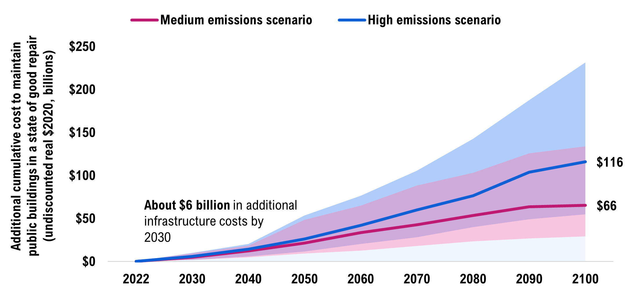
Note: The solid line is the median (or 50th percentile) projection. The coloured bands represent the range of possible outcomes in each emissions scenario. The costs presented in this chart are in addition to the projected baseline costs over the same period.
Source: FAO.
These cumulative costs could vary given the range of climate projections in each global emissions scenario. In the medium emissions scenario, the FAO estimates that by 2100, additional infrastructure-related costs of maintaining Ontario’s public buildings could range from $29 billion (3.7 per cent higher than baseline) to $134 billion (16.8 per cent) by 2100. In the high emissions scenario, these additional costs could range from $55 billion (6.9 per cent) to $232 billion (29 per cent) by 2100.
5 | Adapting public buildings to climate hazards
Chapter 4 described the financial impact of not adapting public buildings to the projected changes in extreme rainfall, extreme heat and freeze-thaw cycles. In practice, buildings can be adapted to withstand these impacts – ensuring that assets perform to the same standards for which they were initially designed and do not suffer accelerated deterioration or higher O&M expenses.
This chapter discusses different forms of adaptation, defines the scope of adaptation analyzed in this report, and estimates a range of costs to adapt Ontario’s portfolio of public buildings to withstand the late-century climate projections for extreme rainfall and extreme heat[34] in the medium and high emissions scenarios.
Adapting public buildings can help prevent the impacts of climate hazards
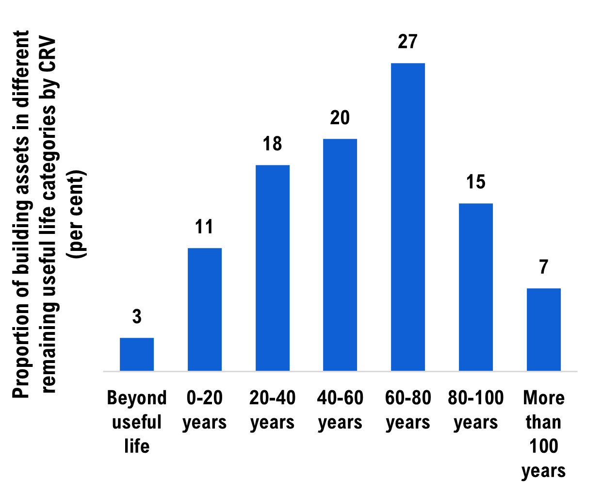
Figure 5-1 Ontario’s public buildings have long remaining useful lives
Source: FAO.
Ontario’s public buildings have very long useful lives. Many buildings constructed in the 19th century are still in use today. Almost 70 per cent of Ontario’s public buildings have a remaining useful life of 40 years or more, and over 20 per cent have a remaining useful life of 80 years or more. Given the long useful lives of public buildings, late-century climate conditions are relevant to adaptation decisions being made now. These decisions will impact public infrastructure costs throughout the century.
However, climate projections depend on the trajectory of global emissions, which remains uncertain. This raises the difficult question of how projected changes in key climate hazards should be accounted for when public buildings are designed, built or retrofitted.[35]
Adapting public infrastructure to extreme rainfall and extreme heat could take many forms. A few examples include:
- Updating infrastructure design parameters to a higher standard.[36]
- Local jurisdictions in Ontario exploring adaptation options and adopting measures, including building code interpretations, general guidance for designers and operators, certification systems, and pilot projects.[37]
- Enhancing the environment around a building to increase its ability to cope with climate hazards. This could be done at large or small scales and involve the use of green infrastructure. For example, the Port Lands Flood Protection Project is expected to provide flood resiliency to 290 hectares of Toronto’s southeastern downtown that sit in the Don River floodplain.[38] To flood protect the Port Lands, the majority of land within the floodplain will be raised by a minimum of one to three metres. The project also incorporates green infrastructure, including the creation of wetlands and marshes, through which water will be directed during very large floods.
- Changing the way assets are managed, for example, changing the frequency of operations and maintenance schedules.[39]
Adaptation can include energy efficiency improvements to help reduce emissions. For example, the federal government is investing $182 million to increase energy efficiency and address climate change by improving how homes and buildings are designed, renovated and constructed. [40]
In the FAO’s framework, adaptation is modelled as an alteration of a building’s physical components to prevent damage costs caused by changes in extreme rainfall and heat. Figure 5-2 presents some examples of adaptation measures for each building component.[41]
Figure 5-2 Examples of building component adaptations to extreme rainfall and extreme heat
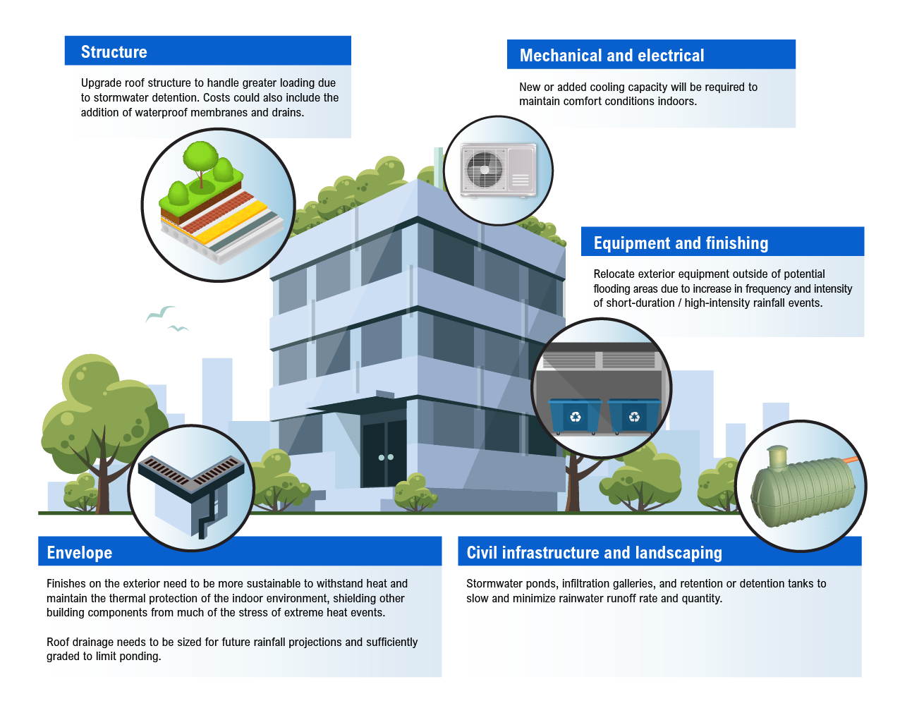
Note: For more examples of how these climate hazards impact building components, see WSP 2021.
Source: WSP.
Adaptation strategy costs vary based on the approach taken
To estimate adaptation costs, the FAO assumed that public buildings and facilities are adapted to withstand the late-century projections[42] for extreme rainfall and extreme heat. Once a building is adapted, the FAO assumes that no additional costs occur from accelerated deterioration or increased O&M expenses.[43] To highlight potential cost differences, the FAO developed two adaptation strategies.
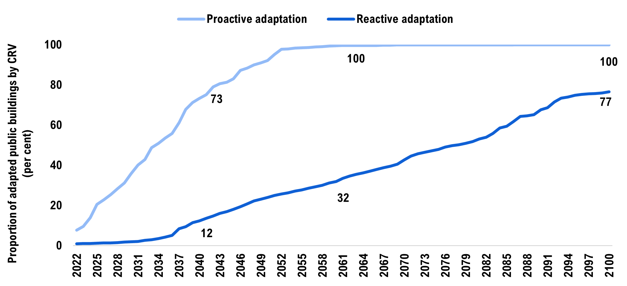
- Reactive adaptation strategy: Buildings are only adapted at the time of renewal. This approach results in a gradual increase in the share of adapted buildings over the century, with roughly 77 per cent of assets adapted by 2100. The remaining 23 per cent have service lives that extend beyond 2100 and are not renewed or adapted over the projection. These buildings incur accelerated deterioration and higher O&M costs over the duration of the outlook.
- Proactive adaptation strategy: Buildings are adapted at the first available opportunity. This occurs either during a building’s next major rehabilitation through a retrofit[44] or at renewal, whichever comes first. In this approach, all buildings are adapted by the 2060s.
Adaptation strategy costs
Costs associated with adaptation strategy include: capital costs from increased deterioration and higher O&M expenses until adaptation, the one-time adaptation expense (either through a retrofit or renewal), and the higher O&M and capital expenses required to maintain higher-valued adapted assets.
Figure 5-3 The reactive adaptation strategy has fewer assets adapted by 2100
Source: FAO.
Adapting Ontario’s public buildings will be expensive
Under the reactive adaptation strategy, maintaining Ontario’s public buildings in a state of good repair would cost an additional $52 billion (6.5 per cent over baseline) cumulatively in the medium emissions scenario to 2100. In the high emissions scenario, the costs would instead increase by $91 billion (11.4 per cent over baseline).
Figure 5-4 The reactive adaptation strategy will see gradual rise in costs throughout the 21st century
Notes: The solid line is the median (or 50th percentile) projection. The coloured bands represent the range of possible outcomes in each emissions scenario. The costs presented in this chart are in addition to the projected baseline costs over the same period.
Source: FAO.
Under the proactive adaptation strategy, maintaining the portfolio would cost an additional $54 billion (6.7 per cent over baseline) cumulatively in the medium emissions scenario to 2100. In the high emissions scenario, the costs would instead increase by $104 billion (13.1 per cent over baseline).[45]
Figure 5-5 Proactively adapting all public buildings would require significant near-term investment
Notes: The solid line is the median (or 50th percentile) projection. The coloured bands represent the range of possible outcomes in each emissions scenario. The costs presented in this chart are in addition to the projected baseline costs over the same period.
Source: FAO.
Under a proactive adaptation strategy, the cumulative costs over the next four decades (2022-2060) are significantly higher compared to the reactive adaptation strategy. This is because all assets are adapted by the 2060s under the proactive strategy while only about one-third of assets are adapted under the reactive strategy by the same period. In addition, most adaptations are done through retrofits, which are more expensive than renewal adaptations.
By the end of the century, the cumulative costs of the proactive strategy are higher than those of the reactive strategy. This reflects the fact that all buildings are adapted under the proactive strategy (many through more expensive retrofits), while under the reactive strategy only 77 per cent of assets are adapted by 2100.[46]
These cumulative costs could vary given the range of climate projections in each global emissions scenario.[47] In the medium emissions scenario, costs across both strategies range from a low of $22 billion (2.8 per cent higher than baseline) to $108 billion (13.5 per cent higher than baseline). In the high emissions scenario, cumulative costs across both strategies range from a low of $44 billion (5.5 per cent higher than baseline) to $174 billion (21.8 per cent higher than baseline).
6 | Comparing the costs of different asset management strategies
Chapters 4 and 5 examined the costs of maintaining assets in a state of good repair in the presence of climate change under three asset management strategies: no adaptation, reactive adaptation and proactive adaptation. None of the strategies presented in this report are meant to be a precise representation of future costs, and the portfolio level costing results are not intended to inform asset-specific management decisions. These strategies were designed to estimate the scale of the budgetary impact that changes in extreme rainfall, extreme heat and freeze-thaw cycles could impose on the province and municipalities over the rest of the century.
This chapter compares cost estimates across the three asset management strategies and discusses the difference in cost profiles between them. The chapter then discusses the factors that were beyond the scope of the FAO’s analysis but are relevant in determining the most cost-effective strategy for managing Ontario’s public buildings in a changing climate.
Adapting public buildings could modestly lower the direct infrastructure costs for the province and municipalities
Changes in extreme rainfall, extreme heat and freeze-thaw cycles will increase the cost of maintaining Ontario’s public buildings in a state of good repair regardless of whether buildings are adapted. However, the timing of when additional costs are incurred as well as the proportion of buildings adapted vary between the different adaptation strategies.
Figure 6‑1 shows how the cumulative cost grows under the three strategies in different emissions scenarios. Under the no adaptation strategy, additional costs accumulate consistently over the projection as extreme rainfall and extreme heat become more frequent and intense. The costs have a similar profile under the reactive adaptation strategy, with savings only starting to take effect after the 2070s.
In contrast, the proactive adaptation strategy sees substantial adaptation costs over the next four decades as all public buildings are adapted primarily through retrofits. This strategy sees much higher up-front costs compared to the no adaptation and reactive strategies. Under this strategy, all public buildings are adapted by the 2060s, leading to a much slower growth in costs in the late century.
Figure 6-1 Asset management strategies to cope with extreme rainfall and heat have different cost profiles
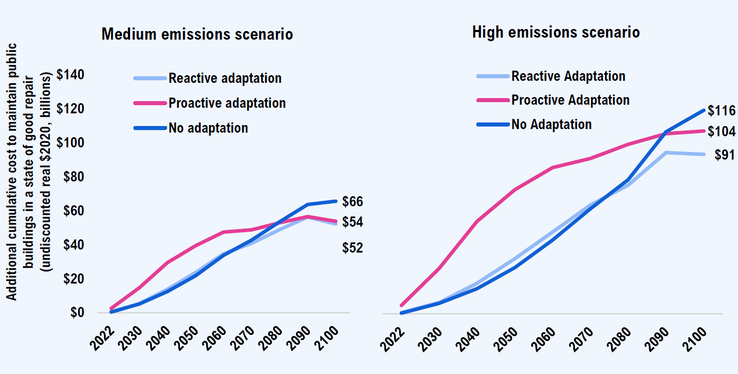
Notes: The solid line is the median (or 50th percentile) projection. The coloured bands represent the range of possible outcomes in each emissions scenario. The costs presented in this chart are in addition to the projected baseline costs over the same period.
Source: FAO.
In both the medium and high emissions scenarios, the FAO estimates that on an undiscounted basis, the cumulative costs by the end of the 21st century are the highest under the no adaptation strategy, followed by the proactive adaptation and reactive adaptation strategies.[48]
Although the differences between the cumulative costs under the three strategies are small relative to the increase in overall costs, the proportion of assets that remain vulnerable to changing climate hazards differs substantially. Under the proactive strategy, 100 per cent of assets are adapted by 2060. Under the reactive strategy, only 32 per cent of assets are adapted by 2060, rising to 77 per cent by the end of the century. Under the no adaptation strategy, all assets remain vulnerable to these changing climate hazards.
Table 6-1 presents a summary of the costs, timing and risk exposure of public buildings under the three different adaptation strategies.
| No Adaptation Strategy | Reactive Adaptation Strategy | Proactive Adaptation Strategy | |
|---|---|---|---|
| When are buildings adapted? | No buildings are adapted | Buildings are adapted during renewal | Buildings are adapted at earliest opportunity |
| What are the additional costs incurred? | Costs from more rapid deterioration and higher O&M expenses | Costs from more rapid deterioration and higher O&M expenses prior to adaptation, costs to adapt assets at renewal, and costs to maintain higher value adapted assets in a state of good repair | Cost from more rapid deterioration and higher O&M expenses prior to adaptation, costs to adapt assets (including one-time retrofits or additional costs at renewal), and costs to maintain higher value adapted assets in a state of good repair |
| What is the timing of these additional costs? | Costs accumulate steadily over the century | Costs accumulate steadily but stabilize near the end of the century as majority of buildings are adapted and avoid costs from accelerated deterioration and higher O&M expenses | Costs increase rapidly to 2060 as all buildings are adapted, then accumulate more slowly as adapted assets avoid costs from accelerated deterioration and higher O&M expenses |
| What is the proportion of adapted buildings by 2100? | No assets are adapted | Roughly 77 per cent of assets are adapted | All assets are adapted |
Other factors should be considered to assess the cost effectiveness of adaptation strategies
Costing of the three different asset management strategies at the portfolio level was designed to estimate the scale of the budgetary impact that changes in extreme rainfall, extreme heat and freeze-thaw cycles could impose on the province and municipalities over the rest of the century. However, to make asset-specific climate adaptation decisions, many other factors should be considered.
Determining the most cost-effective asset management strategy for a specific building would need to account for the asset’s individual characteristics (including age, condition and specific climate vulnerabilities) while balancing other priorities given the government’s budget constraints. A cost-effectiveness analysis would also need to consider a wider array of climate impacts over the entire useful life of an asset than the scope of the FAO’s analysis included.[49]
The following costs and benefits were not included within the FAO’s scope but are likely to have substantial financial impacts.
- More frequent rehabilitations or inspections could potentially disrupt regular service delivery, as would unplanned service disruptions. Such disruptions can impact productivity, community life, health and safety, especially for essential services such as hospitals, schools or water treatment facilities. In extreme cases, severe climate events could leave an asset entirely unusable, significantly impacting the asset owners and users.
- Damage to one part of a building could impact surrounding infrastructure and result in higher financial costs to other asset owners. The FAO’s approach treats the impact of each climate hazard independently and does not account for the significant inter-dependencies between infrastructure components. For example, heavy rainfall may damage a building’s envelope, but the building’s inability to manage the rainfall could also damage surrounding infrastructure.
- Since buildings have long useful lives, adaptation can reduce costs of climate hazards well beyond the 2100 projection horizon. These benefits accruing to the adaptation strategies are not included.
Incorporating these aspects into the analysis would show substantially larger benefits of adaptation.[50]
7 | Appendix
Appendix A : Scope of buildings and facilities analysed
| Level of Government | Sector | Total CRV (2020$ billions) |
Description |
|---|---|---|---|
| Provincial | Transit | $5 |
|
| Hospitals | $45 |
|
|
| Schools | $67 |
|
|
| Colleges | $11 |
|
|
| Other | $13 |
|
|
| Municipal | Transit-related | $2 |
|
| Water-related | $37 |
|
|
| Other buildings and facilities | $75 |
|
Appendix B : Scope of climate variables used in costing analysis
The Canadian Centre for Climate Services provided the projections of all climate indicators used in the FAO’s costing analysis. Depending on the nature of the hazard’s interaction with specific building components, different climate indicators were used. See WSP’s report for a full description and rationale.[52]
| Climate Hazard | Variable | Definition | Low Emissions (RCP2.6) |
Medium Emissions (RCP4.5) |
High Emissions (RCP8.5) |
|---|---|---|---|---|---|
| Extreme Heat | Mean July maximum daily temperature | Monthly mean of daily maximum temperature in July | +1.8°C (+0.9 to 2.5°C) |
+3.6°C (+1.9 to 3.8°C) |
+6.5°C (+4.0 to 7.9°C) |
| 2.5% July daily maximum temperature | 97.5th percentile of the distribution of daily maximum temperature in July | +1.9°C (+0.9 to 2.8°C) |
+3.4°C (+2.4 to 4.3°C) |
+6.5°C (+4.3 to 7.6°C) |
|
| Annual number of cooling degree-days | Annual sum of daily degrees above 18°C | +71°C-days (+37 to 117°C-days) |
+161°C-days (+86 to 212°C-days) |
+381°C-days (+225 to 515°C-days) |
|
| Extreme Rainfall | Annual total precipitation | Annual total amount of precipitation received | +7.1 per cent (+4.0 to 7.8 per cent) |
+9.8 per cent (+4.4 to 10.3 per cent) |
+15.0 per cent (+6.2 to 18.2 per cent) |
| IDF 15-min 1:10 | Short duration rainfall intensity for a 15-minute 1-in-10-year event | +14.6 per cent (+9.8 to 23.5 per cent) |
+24.9 per cent (+16.1 to 39.4 per cent) |
+53.0 per cent (+38.0 to 78.2 per cent) |
|
| IDF 24-hour 1:5 | Short duration rainfall intensity for a 24-hour 1-in-5-year event | +14.6 per cent (+9.8 to 23.5 per cent) |
+24.9 per cent (+16.1 to 39.4 per cent) |
+53.0 per cent (+38.0 to 78.2 per cent) |
|
| IDF 24-hour 1:100 | Short duration rainfall intensity for a 24-hour 1-in-100-year event | +14.6 per cent (+9.8 to 23.5 per cent) |
+24.9 per cent (+16.1 to 39.4 per cent) |
+53.0 per cent (+38.0 to 78.2 per cent) |
|
| IDF 24-hour 1:10 | Short duration rainfall intensity for a 24-hour 1-in-10-year event | +14.6 per cent (+9.8 to 23.5 per cent) |
+24.9 per cent (+16.1 to 39.4 per cent) |
+53.0 per cent (+38.0 to 78.2 per cent) |
|
| Freeze-Thaw Cycles | Annual freeze-thaw cycles | Annual number of days with daily maximum temperature above 0°C and daily minimum temperature below 0°C | -5.5 per cent (-15.2 to 0.0 per cent) |
-12.1 per cent (-19.2 to 0.0 per cent) |
-15.1 per cent (-24.9 to 0.0 per cent) |
| Deep freeze-thaw cycles | Annual number of days with daily maximum temperature above 0°C, daily minimum temperature below 0°C, and daily average temperature equal or less than 0°C | -2.3 per cent (-8.3 to +4.6 per cent) |
-4.4 per cent (-10.8 to +4.8 per cent) |
-4.9 per cent (-15.8 to +12.5 per cent) |
Appendix C : The impact of climate hazards on public buildings
In the absence of adaptation measures, changes in extreme rainfall, extreme heat and freeze-thaw cycles will impact the useful service life (USL) of public buildings. They will also impact the operations and maintenance (O&M) spending that would be required to maintain Ontario’s portfolio of public buildings in a state of good repair. However, adapting public buildings to withstand changes in these climate hazards will require investment.
To establish relationships between relevant climate indicators and key infrastructure costs, the FAO worked with WSP, a large engineering firm with expertise in all aspects of public sector infrastructure, including asset management, public infrastructure construction and operations, and climate change impacts. WSP estimated relationships between climate variables and infrastructure costs by surveying relevant engineering experts. To account for engineering uncertainty, WSP aggregated their responses and provided optimistic, pessimistic and most-likely cost relationships. This forms the basis on which the FAO estimated the additional costs of climate hazards to public buildings in Ontario.[53]
Based on these engineering relationships, this appendix describes how the three climate hazards are expected to impact the USL and O&M costs of Ontario’s public buildings over the rest of the 21st century. It also provides average adaptation cost estimates to adapt public buildings to the projected change in these climate hazards for each decade of the century.
While regional climate projections were used to develop the FAO’s cost estimates, the results presented in this appendix combine Ontario average climate projections with WSP’s cost relationships to illustrate the impacts. The engineering impacts by economic regions are available on the FAO website.
Climate hazards are reducing the useful service life of public buildings in the absence of adaptation
The FAO estimates that increases in extreme rainfall and heat are reducing the USL of public buildings in Ontario, resulting in faster deterioration than would otherwise have occurred in a stable climate. Over the long term, increases in extreme rainfall and heat will further reduce the USL of buildings in both emissions scenarios, although the impact is more significant in the high emissions scenario. While impacts to individual buildings may vary, these results should be interpreted as the average impact across the portfolio of public buildings in the project’s scope.
Figure 7-1 The useful service life of public buildings will decline due to projected changes in extreme heat, extreme rainfall and freeze-thaw cycles in the absence of adaptation actions
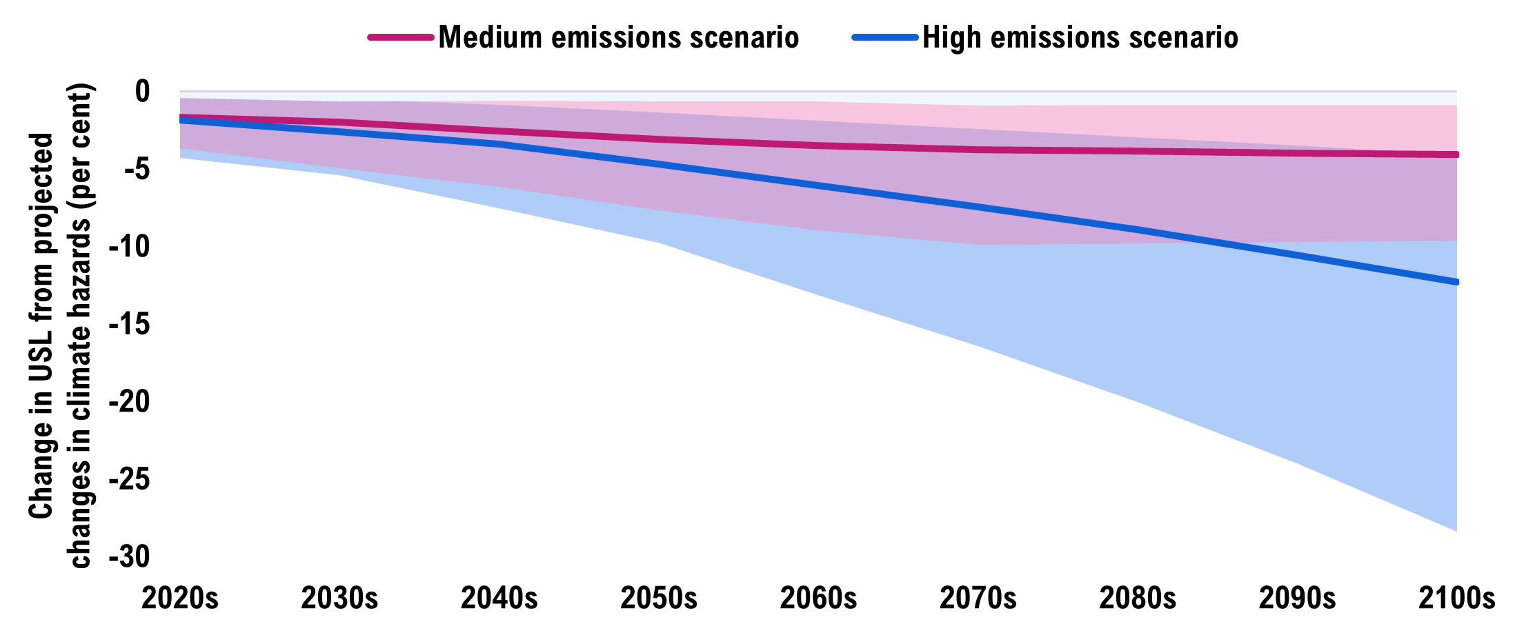
Note: The solid line is the median (or 50th percentile) climate projection using “most likely” engineering outcomes. The coloured bands represent the range of possible outcomes in each emissions scenario given climate and engineering uncertainty.
Source: WSP and FAO.
Trends in extreme rainfall primarily drive the reduction in USL for Ontario’s portfolio of public, followed by extreme heat. While declining trends in freeze-thaw cycles are estimated to prolong USLs, this is more than offset by the impact of the other hazards.
Figure 7-2 More extreme rainfall is the biggest factor accelerating the deterioration of public buildings
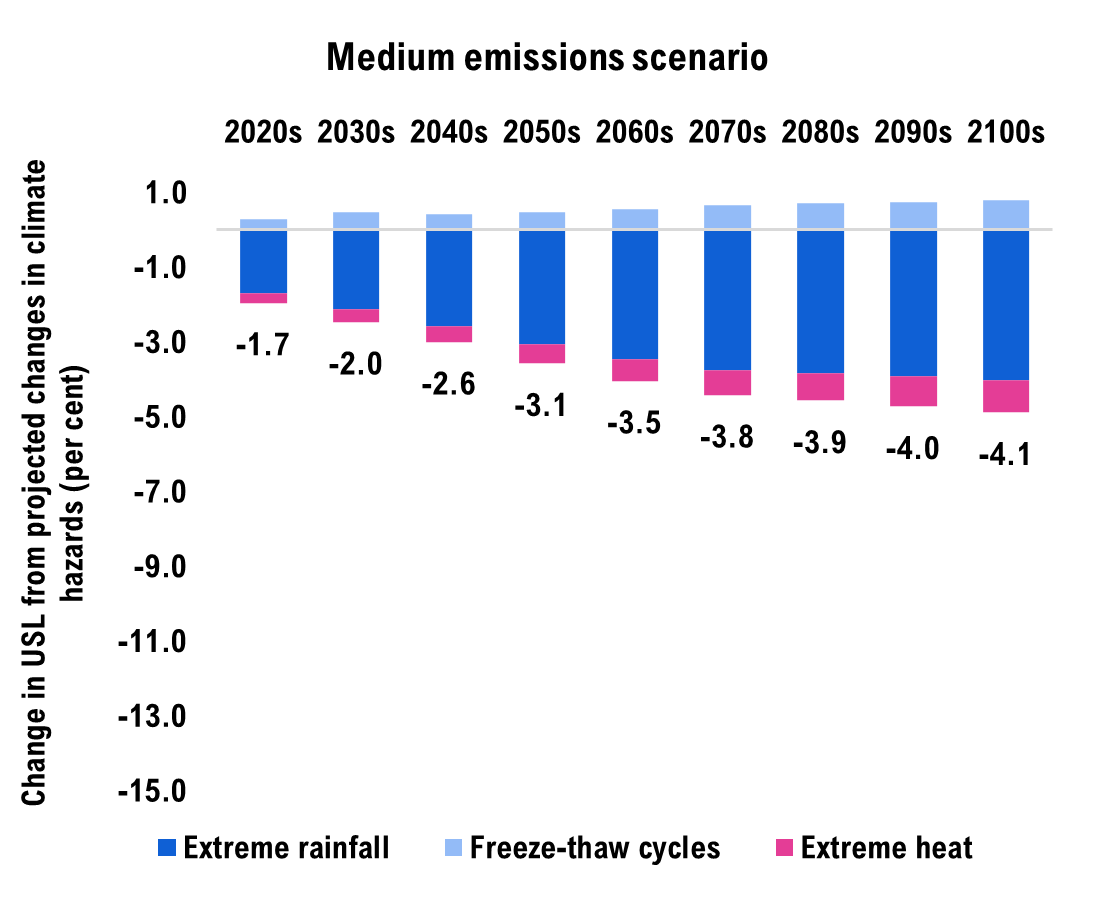
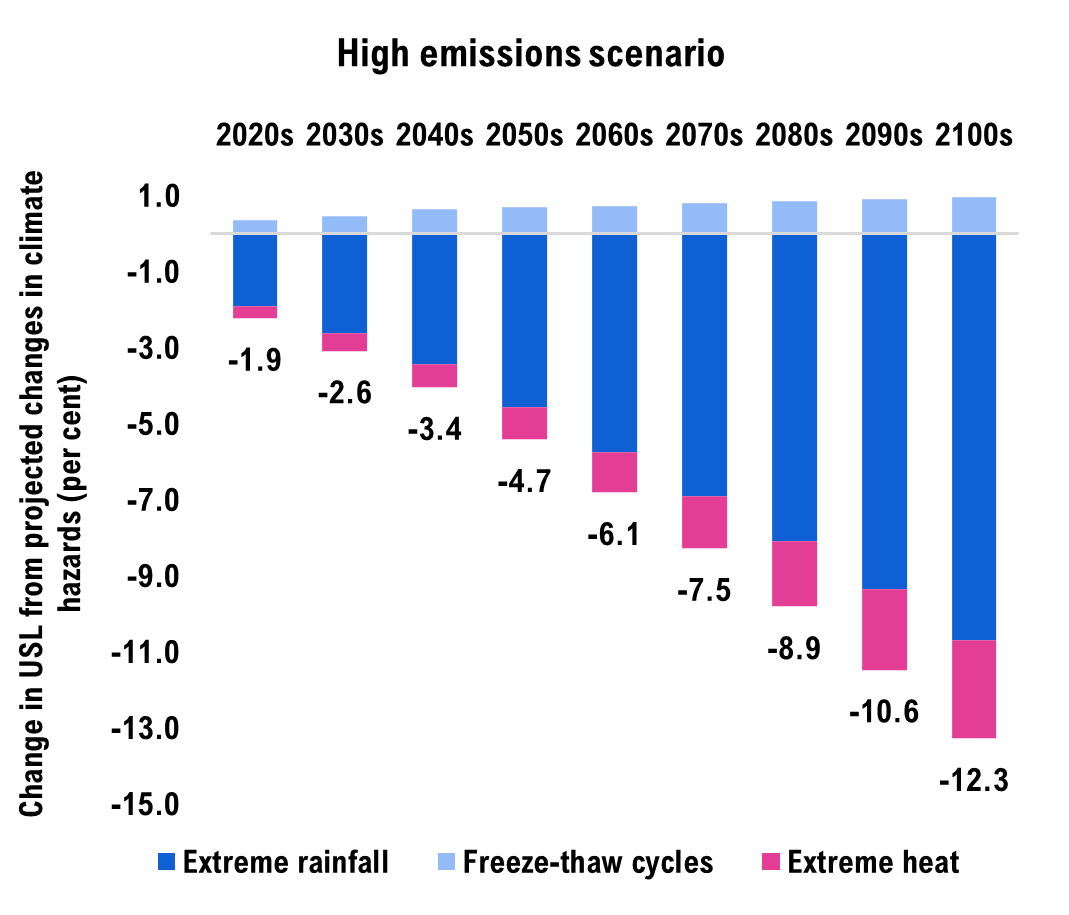
Note: These values are based on the median (50th percentile) Ontario average climate projections using the estimates of “most likely” engineering outcome. The range of climate and engineering uncertainties has been omitted in this figure for presentation purposes.
Source: WSP and FAO.
Climate hazards will increase O&M expenses for public buildings in the absence of adaptation
The FAO estimates that increases in extreme rainfall and heat are raising the O&M expenses of public buildings faster than would otherwise have occurred in a stable climate. Over the rest of the century, the required O&M expense to maintain public buildings in a state of good repair is projected to rise in both emissions scenarios, with a larger increase in the high emissions scenario.
Figure 7-3 Projected changes in extreme rainfall, extreme heat and freeze-thaw cycles will raise the O&M expenses of Ontario’s public buildings in the absence of adaptation actions
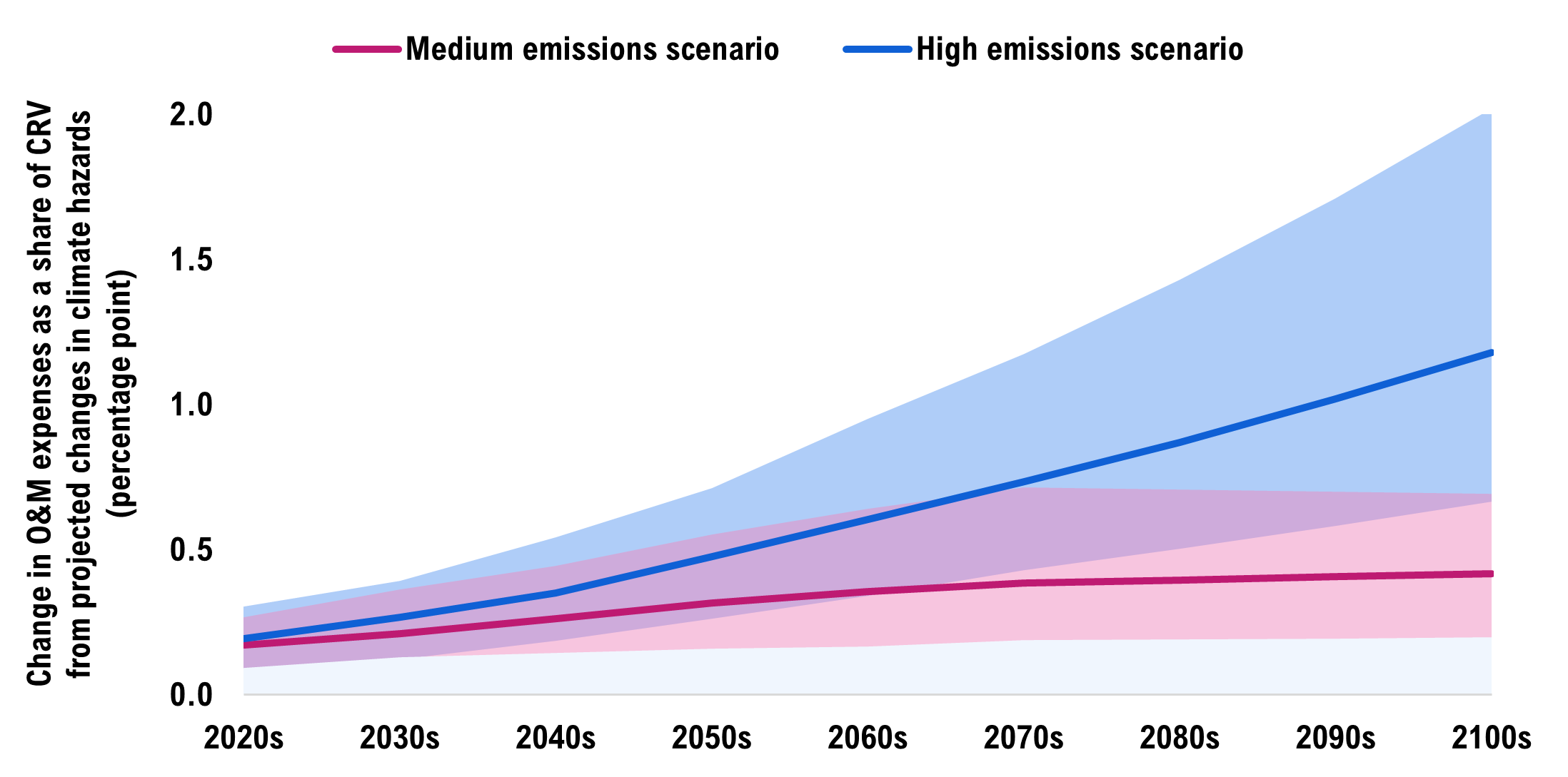
Note: The solid line is the median (or 50th percentile) climate projection using “most likely” engineering outcomes. The coloured bands represent the range of possible outcomes in each emissions scenario given climate and engineering uncertainty.
Source: WSP and FAO.
Trends in extreme rainfall are expected to drive most of the projected increases in O&M expenses to public buildings, while extreme heat has a much smaller impact. Fewer freeze-thaw cycles in the future will modestly reduce O&M expenses to public buildings on average, although the impacts of other hazards more than offset this small reduction.
Figure 7-4 More intense rainfall will contribute the most to rising O&M costs for public buildings
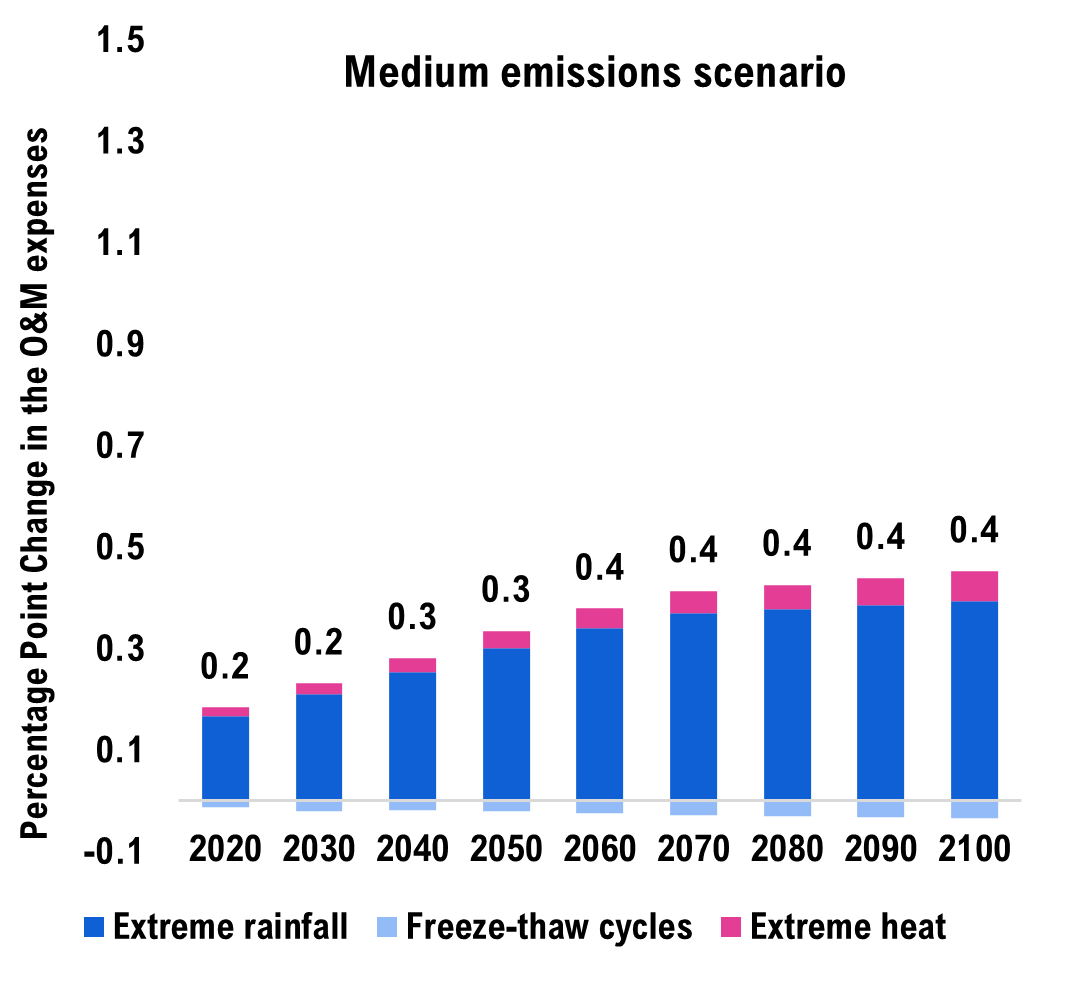
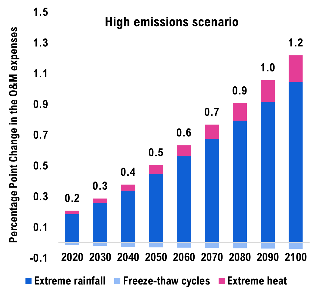
Note: These values are based on the median (50th percentile) Ontario average climate projections using the estimates of “most likely” engineering outcome. The range of climate and engineering uncertainties has been omitted in this figure for presentation purposes.
Source: WSP and FAO.
The cost of adapting public buildings to withstand these climate hazards increases with the extent of climate change
In the FAO’s framework, adaptation is modelled as an alteration of a building’s physical components to prevent more rapid deterioration and increased O&M expenses caused by changes in extreme rainfall and heat. Adaptation costs are considered one-time investments, occurring either as a retrofit during a building’s service life, or as part of a full redesign and rebuild at the end of its service life.
The costs of adaptation are also assumed to vary depending on the severity of the climate hazards the adaptation is designed to withstand. The more severe the climate hazard, the higher the expected adaptation costs. Based on WSP estimates, the cost of adapting a building during its service life through a retrofit is expected to be more expensive than the increased cost of designing and constructing a new climate-adapted building at the end of its service life.
While the FAO’s analysis only uses the cost estimates in the 2080s to estimate portfolio-wide adaptation costs, the full range of costs per decade is shown below to illustrate how these costs vary with changing climate hazards. Adaptation costs are expressed as a percentage of a building’s current replacement value. For example, if a building is valued at $1.0 million, and the adaptation is assumed to cost 5 per cent, the adaptation cost is $50,000. All costs are in 2020 real dollars.
Figure 7-5 The cost of retrofitting Ontario’s public buildings to withstand extreme rainfall and heat will depend on the extent of climate change
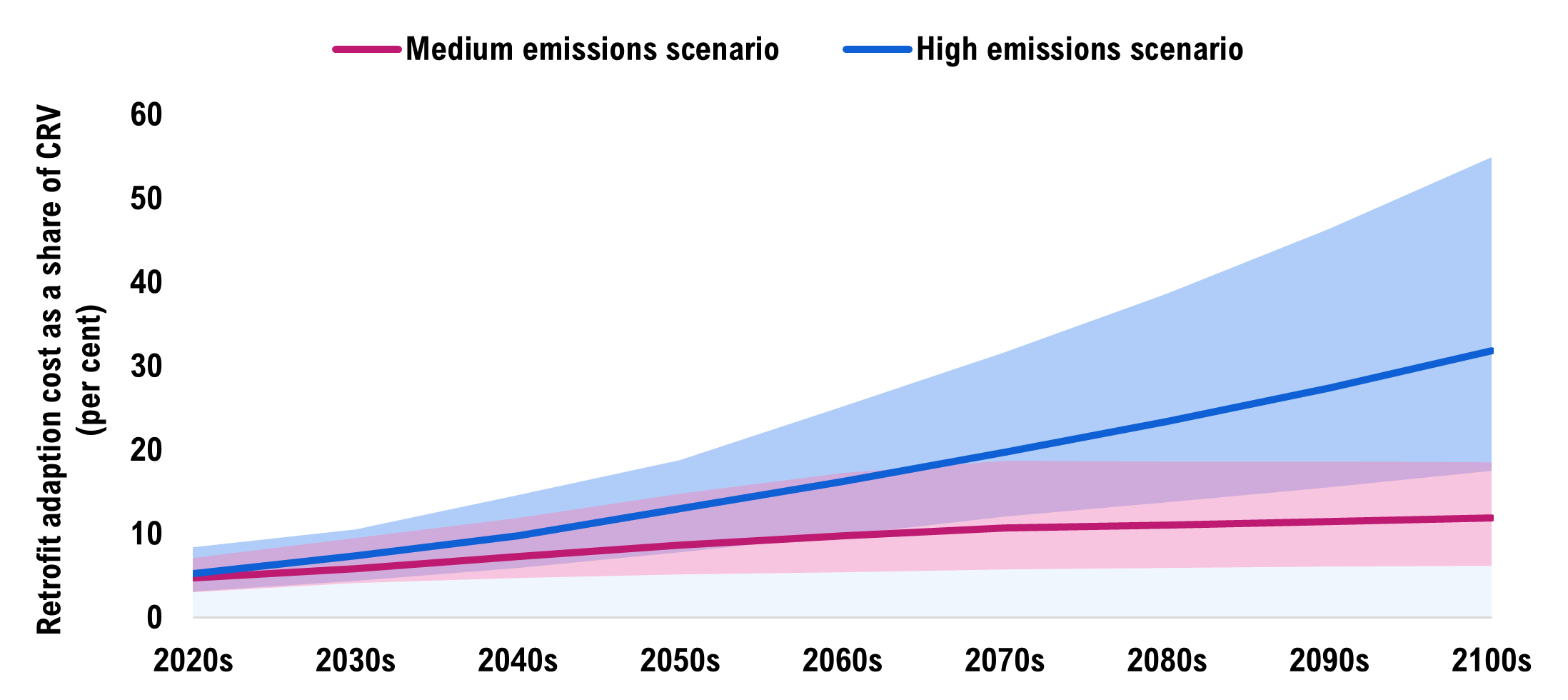
Note: The solid line is the median (or 50th percentile) climate projection using “most likely” engineering outcomes. The coloured bands represent the range of possible outcomes in each emissions scenario given climate and engineering uncertainty.
Source: WSP and FAO.
Figure 7-6 The cost of adapting Ontario’s public buildings at renewal to withstand extreme rainfall and heat will depend on the extent of climate change
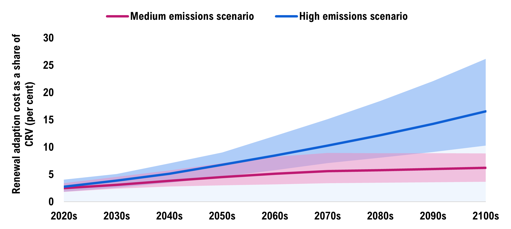
Note: The solid line is the median (or 50th percentile) climate projection using “most likely” engineering outcomes. The coloured bands represent the range of possible outcomes in each emissions scenario given climate and engineering uncertainty.
Source: WSP and FAO.
Appendix D : Comparing the present value costs of different asset management strategies
When evaluating financial decisions, the timing of cash flows is important.[54] A standard approach to deal with the timing implications of spending is to discount costs into present value dollars using a discount rate. When discounted, costs incurred further in the future carry less weight relative to costs incurred sooner.
Chapter 6 showed that in undiscounted real dollars, the reactive adaptation strategy had a marginally lower cumulative additional cost over the projection, followed by the proactive adaptation strategy, while the no adaptation strategy had the highest costs. Figure 7-7 shows how the choice of discount rate impacts the present value of the total cost estimates for the median climate projections.
Figure 7-7 The present value cost of each asset management strategy under different discount rates
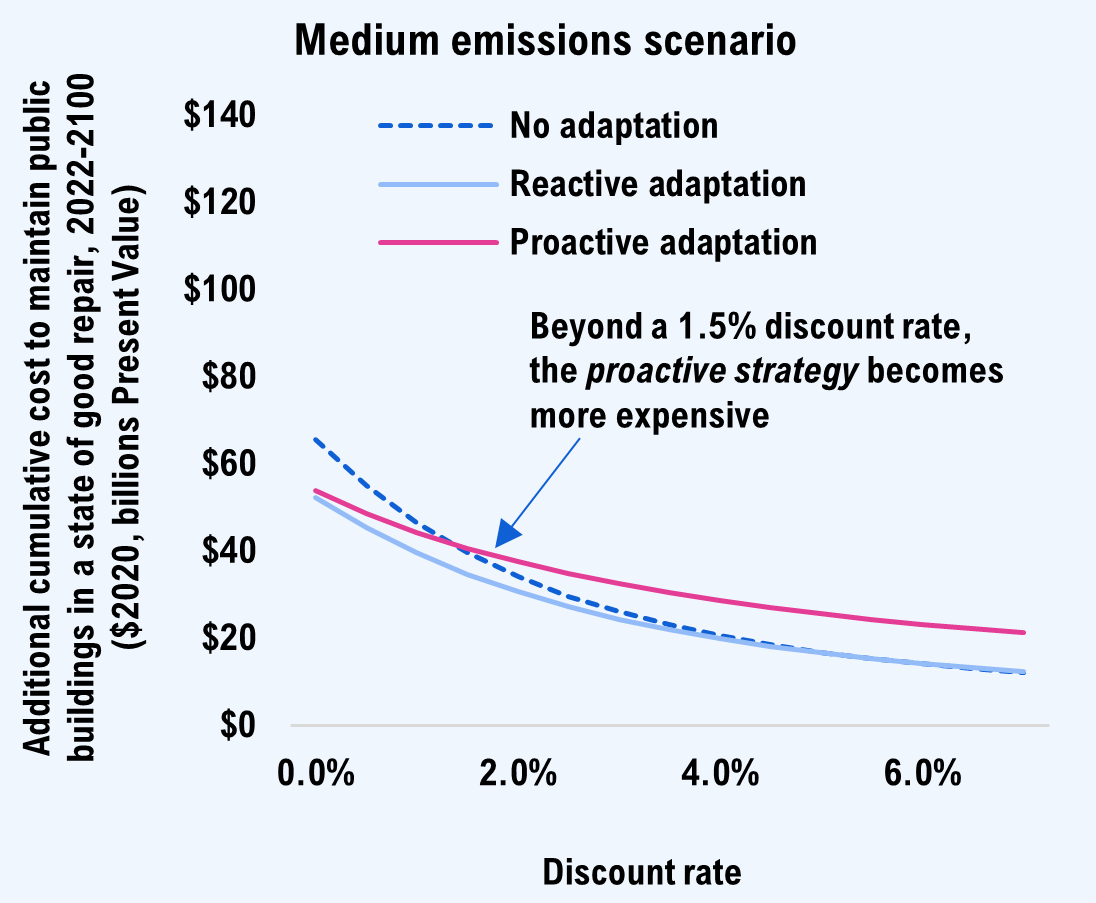
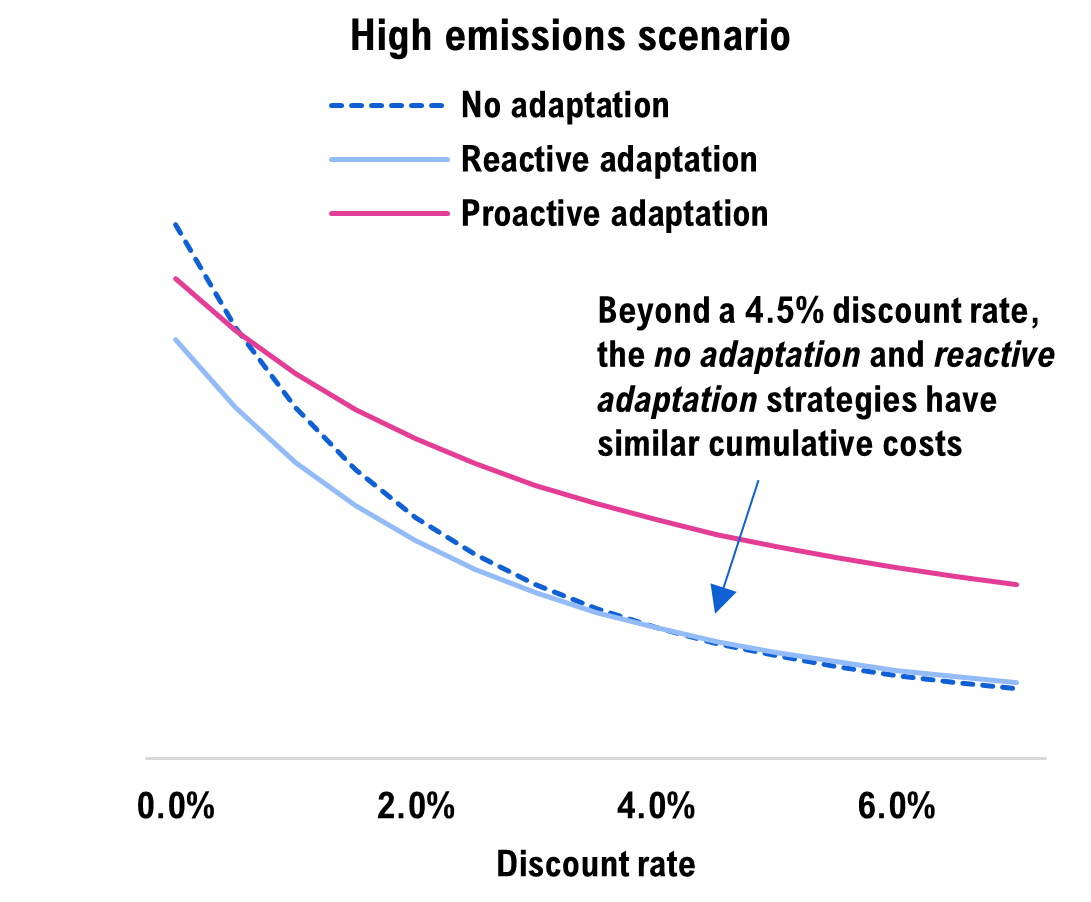
Note: The costs presented use the median (50th percentile) climate projections and “most likely” engineering costs.
Source: FAO.
At discount rates above 1 or 1.5 per cent (depending on the emissions scenario), the proactive adaptation strategy is more expensive in present value terms compared to other strategies. At discount rates below 4.5 to 5.5 per cent, the reactive adaptation strategy remains the lower cost strategy in present value terms. However, above 4.5 to 5.5 per cent, the present value of the reactive adaptation and no adaptation strategies becomes similar. This happens as the cost profiles under both strategies are comparable until 2070s (see Figure 6‑1), and the savings from the reactive adaptation strategy after 2070s are more heavily discounted at higher rates.
The choice of a discount rate will affect the relative costs of each strategy. Rate selection will have intergenerational equity implications, as higher discount rates favour current generations over future ones. These strategies were not designed to inform asset-specific management decisions, but rather to estimate the scale of their budgetary impacts. The costs compared above do not incorporate the full spectrum of societal impacts these climate hazards will impose (as noted in Chapter 6), nor do they reflect the climate and engineering uncertainties discussed throughout the report.
Appendix E : Costing results in the low emissions scenario
While the report focused on the medium and high emissions scenario, Appendix E presents the costing results of the three adaptation strategies for all emissions scenarios.
In the low emissions scenario, a major and immediate turnaround in global climate policies is assumed. Emissions are projected to peak in the early 2020s and decline to zero by the 2080s, limiting the rise in global mean temperatures to 1.6°C (0.8 to 2.4°C) by 2100 compared to the pre-industrial average.[55] Even in the low emissions scenario, change in extreme rainfall, extreme heat and freeze-thaw cycles will still have material financial impacts. Taken together they would raise the costs of maintaining Ontario’s public buildings by $43 billion (5.4 per cent above baseline) to 2100 in the absence of adaptation.
Figure 7-8 More extreme rainfall and heat will raise the cost of maintaining the current portfolio of public buildings by $43 billion in the low emissions scenario in the absence of adaptation
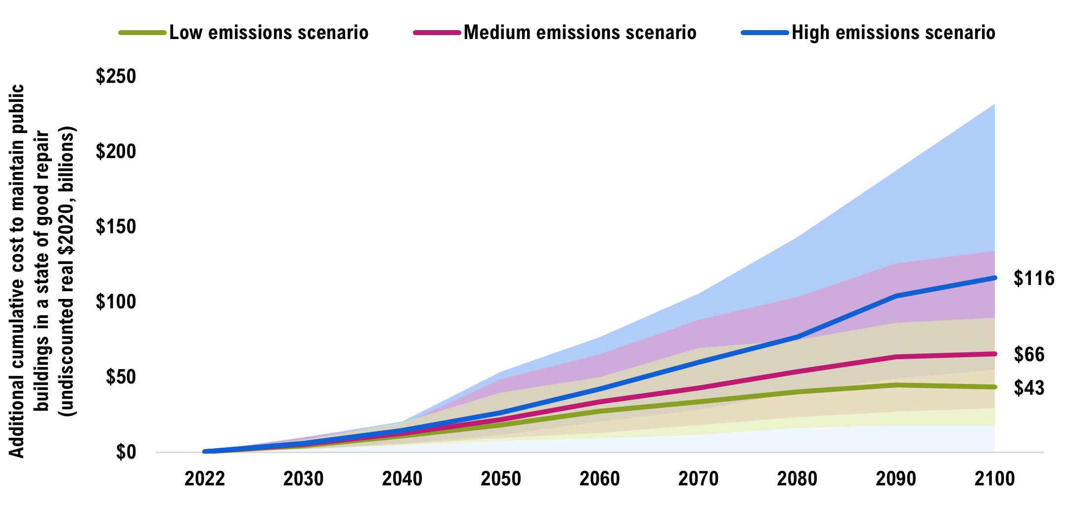
Note: The solid line is the median (or 50th percentile) projection. The coloured bands represent the range of possible outcomes in each emissions scenario. The costs presented in this chart are in addition to the projected baseline costs over the same period.
Source: WSP and FAO.
Figure 7-9 A reactive adaptation strategy, where buildings are adapted when renewed at the end of their service life to withstand the impacts of more extreme rainfall and heat, will add $35 billion in infrastructure costs over the century in the low emissions scenario
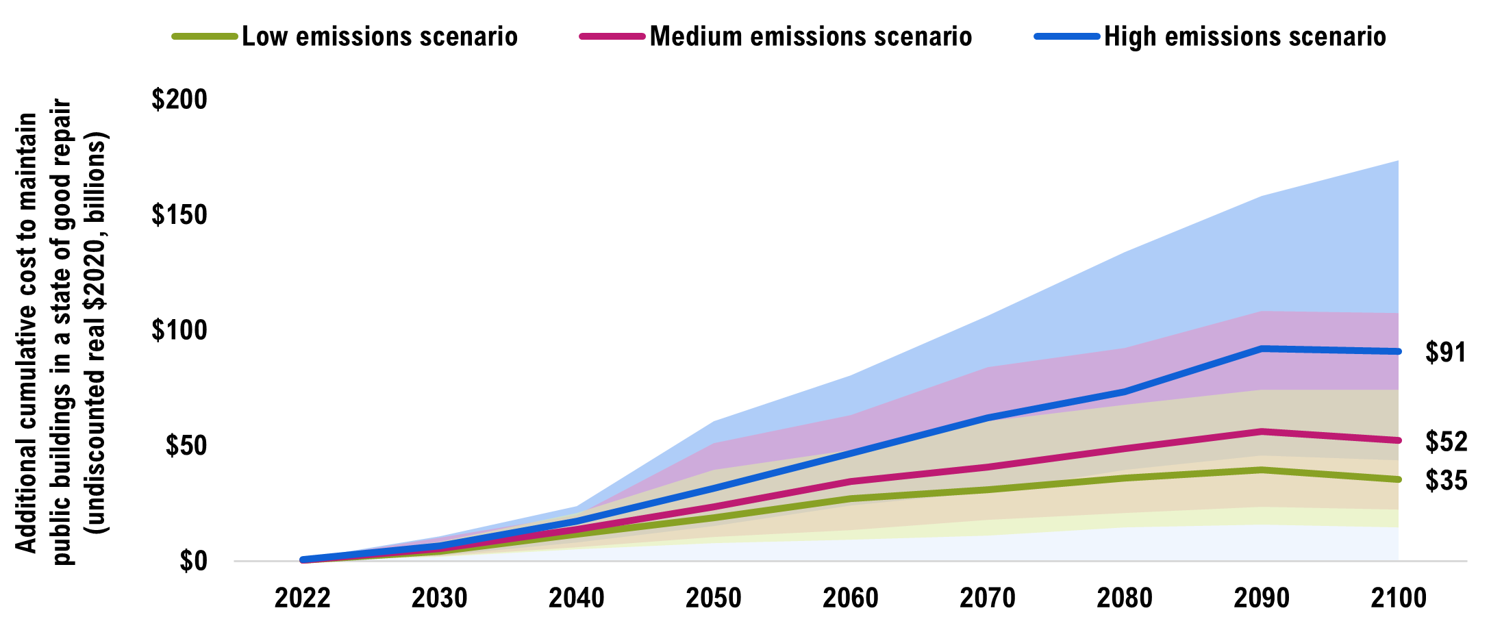
Note: The solid line is the median (or 50th percentile) projection. The coloured bands represent the range of possible outcomes in each emissions scenario. The costs presented in this chart are in addition to the projected baseline costs over the same period.
Source: WSP and FAO.
Figure 7-10 A proactive adaptation strategy, where buildings are adapted at the earliest opportunity to withstand the impacts of more extreme rainfall and heat, will add $33 billion in infrastructure costs over the century in the low emissions scenario
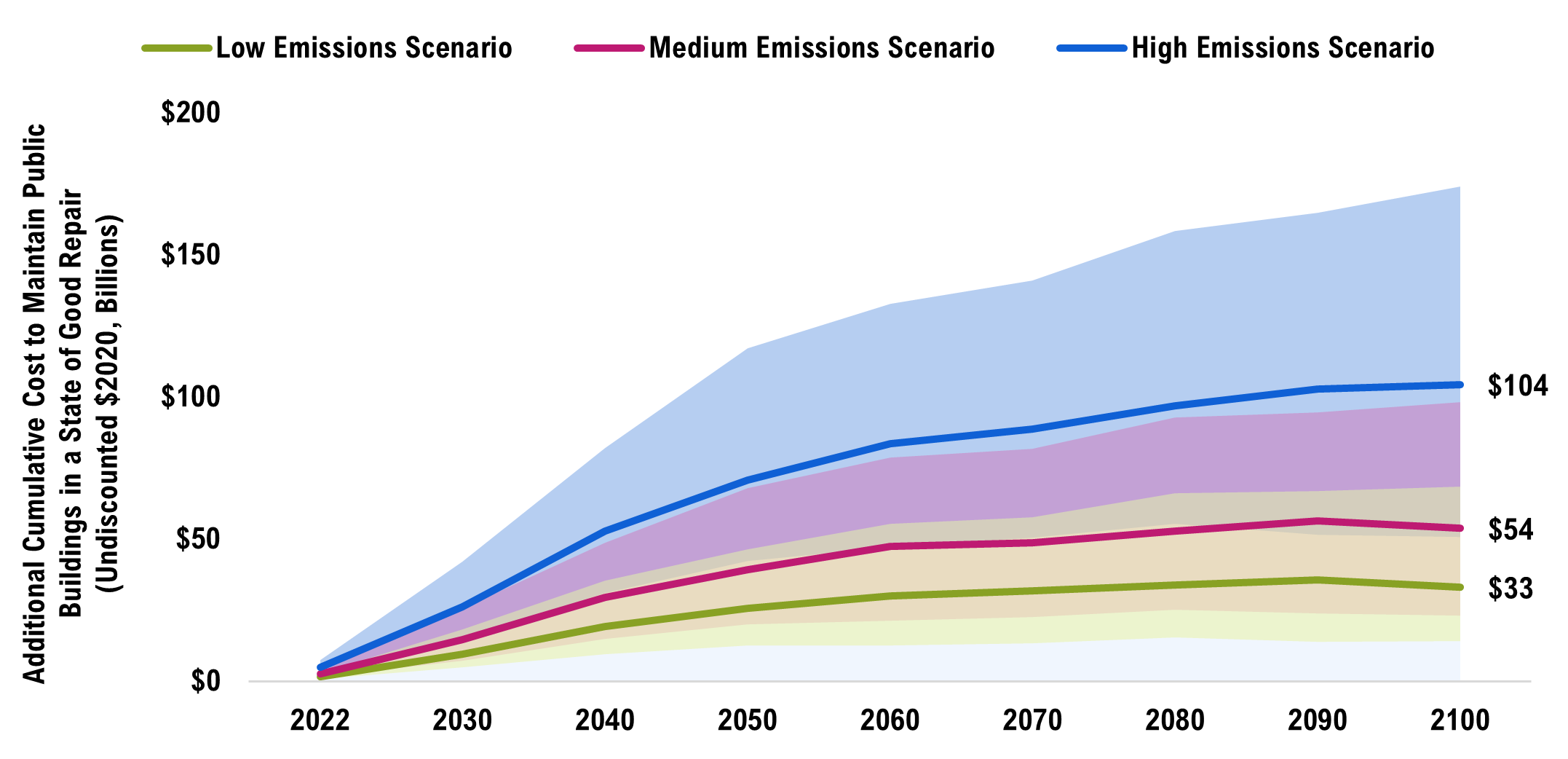
Note: The solid line is the median (or 50th percentile) projection. The coloured bands represent the range of possible outcomes in each emissions scenario. The costs presented in this chart are in addition to the projected baseline costs over the same period.
Source: WSP and FAO.
8 | References
- Asset Management BC. Climate Change and Asset Management: A Sustainable Service Delivery Primer.
- Financial Accountability Office of Ontario, 2020, Provincial Infrastructure.
- Financial Accountability Office of Ontario, 2021a, Municipal Infrastructure.
- Financial Accountability Office of Ontario, 2021b, Costing Climate Change Impacts to Public Infrastructure: Project Backgrounder and Methodology.
- Government of Canada, 2019. Infrastructure Canada’s Climate Lens.
- Government of Canada, 2021. Natural Resources Canada Canada’s Climate Change Adaptation Platform.
- Government of Canada, 2020. Natural Resources Canada Energy Efficient Buildings RD&D
- Institute for Catastrophic Loss Reduction, 2020, Estimating the benefits of Climate Resilient Buildings and Core Public Infrastructure (CRBCPI)
- Intergovernmental Panel on Climate Change, 2013, Climate Change 2013: The Physical Science Basis: Annex II: Climate System Scenario Tables.
- Intergovernmental Panel on Climate Change, 2021, Climate Change 2021: The Physical Science Basis: Summary for Policymakers.
- Intergovernmental Panel on Climate Change, 2014, Climate Change 2014: Impacts, Adaptation, and Vulnerability, Chapter 14: Economics of Adaptation.
- International Institute of Sustainable Development, 2021, Advancing the Climate Resilience of Canadian Infrastructure: A review of literature to inform the way forward.
- National Research Council of Canada, 2015. National Building Code of Canada 2015.
- Neumann, J.E., Chinowsky, P., Helman, J.et al., 2021, Climate effects on US infrastructure: the economics of adaptation for rail, roads, and coastal development.Climatic Change167,44.
- Ontario Ministry of Municipal Affairs, 2016. 2012 Building Code Compendium Volume 1. January 1, 2017 update.
- Organization for Economic Cooperation and Development (OECD), 2018. Climate-Resilient Infrastructure.
- Pacific Climate Impacts Consortium, 2021, PCIC Science Brief: Should the RCP 8.5 emissions scenario represent “business as usual?”.
- Warren, F. and Lulham, N., editors, 2021, Canada in a Changing Climate: National Issues Report, Government of Canada.
- Waterfront Toronto, 2021. Port Lands Flood Protection Project.
- United Nations Environment Program (UNEP), 2021, Buildings and Climate Change Adaptation: A Call to Action.
- United Nations Framework Convention on Climate Change, 2011, Assessing the Costs and Benefits of Adaptation Options.
- WSP, 2021, Costing climate change impacts and adaptation for provincial and municipal public infrastructure in Ontario, Deliverable #10 – Final Report, Toronto, Ontario. Report produced for Financial Accountability Office of Ontario.
| Release Date | Report Title |
|---|---|
| Previously Released | Provincial Infrastructure |
| Municipal Infrastructure | |
| Fall 2021 | CIPI Project Backgrounder and Methodology |
| WSP Report | |
| Buildings and Facilities | |
| 2022 | Public Transportation Infrastructure |
| Public Water Infrastructure | |
| Summary Report |
| Emissions Scenario | 2022 | 2030 | 2040 | 2050 | 2060 | 2070 | 2080 | 2090 | 2100 | |
|---|---|---|---|---|---|---|---|---|---|---|
| Medium | Low | $0 | $2 | $5 | $9 | $13 | $18 | $24 | $27 | $29 |
| Median | $0 | $5 | $12 | $22 | $34 | $43 | $54 | $64 | $66 | |
| High | $1 | $10 | $19 | $49 | $65 | $88 | $103 | $126 | $134 | |
| High | Low | $0 | $2 | $6 | $12 | $20 | $28 | $40 | $49 | $55 |
| Median | $0 | $6 | $14 | $26 | $42 | $60 | $77 | $104 | $116 | |
| High | $1 | $10 | $20 | $54 | $77 | $106 | $143 | $188 | $232 |
| Medium Emissions Scenario | High Emissions Scenario | |
|---|---|---|
| No Adaptation | $66 | $116 |
| Reactive Adaptation | $52 | $91 |
| Proactive Adaptation | $54 | $104 |
| Level of Government | Sector | CRV | Share |
|---|---|---|---|
| Municipal | Other buildings and facilities | $75 | 29% |
| Potable water, Storm water and Wastewater Facilities | $37 | 14% | |
| Transit | $2 | 1% | |
| Provincial | Schools | $67 | 26% |
| Hospitals | $45 | 18% | |
| Other provincial buildings | $13 | 5% | |
| Colleges | $11 | 4% | |
| Transit | $5 | 2% |
| Year | Proportion of Public Building Infrastructure by CRV Requiring Rehabilitation and Renewal Spending (Per Cent) | Average |
|---|---|---|
| 2022 | 8 | 6 |
| 2023 | 1 | |
| 2024 | 2 | |
| 2025 | 4 | |
| 2026 | 7 | |
| 2027 | 2 | |
| 2028 | 5 | |
| 2029 | 3 | |
| 2030 | 4 | |
| 2031 | 3 | |
| 2032 | 4 | |
| 2033 | 3 | |
| 2034 | 7 | |
| 2035 | 4 | |
| 2036 | 5 | |
| 2037 | 7 | |
| 2038 | 8 | |
| 2039 | 9 | |
| 2040 | 10 | |
| 2041 | 5 | |
| 2042 | 6 | |
| 2043 | 5 | |
| 2044 | 4 | |
| 2045 | 4 | |
| 2046 | 5 | |
| 2047 | 11 | |
| 2048 | 7 | |
| 2049 | 4 | |
| 2050 | 6 | |
| 2051 | 8 | |
| 2052 | 8 | |
| 2053 | 11 | |
| 2054 | 8 | |
| 2055 | 5 | |
| 2056 | 3 | |
| 2057 | 6 | |
| 2058 | 5 | |
| 2059 | 3 | |
| 2060 | 6 | |
| 2061 | 9 | |
| 2062 | 7 | |
| 2063 | 6 | |
| 2064 | 6 | |
| 2065 | 3 | |
| 2066 | 6 | |
| 2067 | 9 | |
| 2068 | 10 | |
| 2069 | 4 | |
| 2070 | 4 | |
| 2071 | 8 | |
| 2072 | 5 | |
| 2073 | 7 | |
| 2074 | 5 | |
| 2075 | 8 | |
| 2076 | 4 | |
| 2077 | 4 | |
| 2078 | 4 | |
| 2079 | 4 | |
| 2080 | 8 | |
| 2081 | 10 | |
| 2082 | 5 | |
| 2083 | 3 | |
| 2084 | 5 | |
| 2085 | 4 | |
| 2086 | 7 | |
| 2087 | 4 | |
| 2088 | 4 | |
| 2089 | 13 | |
| 2090 | 5 | |
| 2091 | 4 | |
| 2092 | 6 | |
| 2093 | 5 | |
| 2094 | 4 | |
| 2095 | 7 | |
| 2096 | 5 | |
| 2097 | 6 | |
| 2098 | 9 | |
| 2099 | 10 | |
| 2100 | 3 |
| Building Component | Includes | Relevant climate hazards |
|---|---|---|
| Structure | Superstructure, foundation, and roof structure. | Humidity and freeze-thaw cycles impact the structure if cracks in the material are present. Greatest impact is likely to be experienced in exposed components where water accumulation is most likely. |
| Mechanical and Electrical | Boilers, air terminal AV box, ductwork, roof top air conditioner, panel board, motors, conduits, and wiring. | Extreme heat impacts mechanical and electrical systems, depending on the thermal isolation of the envelope and on the capacity of mechanical systems to maintain ambient air in specific conditions (temperature and humidity). |
| Equipment and Finishing | Painting, high-performance coatings, and staining, parking control, loading docks, and waste-handling. | Extreme rainfall and freeze-thaw cycles impact equipment and finishing, depending on the performance of the envelope. Exposure of interior finishes to leakage may result in mold development and impact the durability of the assets. |
| Envelope | Claddings, doors, glazing, and roof. | Extreme high temperature fosters thermal expansion of materials and decreasing building performance. Freeze-thaw cycles cause envelope deterioration and cracking. Extreme rainfall results in erosion of porous materials, corrosion, and damage from leakage. |
| Civil and Landscaping | Asphalt, concrete walkways and surfacing. | Extreme rainfall undermines the performance of water management systems—the primary civil infrastructure component of buildings. Extreme heat and freeze-thaw cycles impact the asphalt and concrete elements. |
| Emissions Scenario | Damage | 2022 | 2030 | 2040 | 2050 | 2060 | 2070 | 2080 | 2090 | 2100 |
|---|---|---|---|---|---|---|---|---|---|---|
| Medium | Low | $0 | $2 | $5 | $9 | $13 | $18 | $24 | $27 | $29 |
| Median | $0 | $5 | $12 | $22 | $34 | $43 | $54 | $64 | $66 | |
| High | $1 | $10 | $19 | $49 | $65 | $88 | $103 | $126 | $134 | |
| High | Low | $0 | $2 | $6 | $12 | $20 | $28 | $40 | $49 | $55 |
| Median | $0 | $6 | $14 | $26 | $42 | $60 | $77 | $104 | $116 | |
| High | $1 | $10 | $20 | $54 | $77 | $106 | $143 | $188 | $232 |
| Remaining useful life categories | Proportion of building assets in different remaining useful life categories by CRV (Per Cent) |
|---|---|
| Beyond Useful Life | 3 |
| 0-20 years | 11 |
| 20-40 years | 18 |
| 40-60 years | 20 |
| 60-80 years | 27 |
| 80-100 years | 15 |
| More than 100 years | 7 |
| Civil and Landscaping | Stormwater ponds, infiltration galleries, and retention or detention tanks to slow and minimize rainwater runoff rate and quantity. |
|---|---|
| Structure | Upgrade roof structure to handle greater loading due to stormwater detention. Costs could also include the addition of waterproof membranes and drains. |
| Envelope | Finishes on the exterior need to be more sustainable to withstand heat and maintain the thermal protection of the indoor environment, shielding other building components from much of the stress of extreme heat events. Roof drainage needs to be sized for future rainfall projections and sufficiently graded to limit ponding. |
| Mechanical and Electrical | New or added cooling capacity will be required to maintain comfort conditions indoors. |
| Equipment and Finishing | Relocate exterior equipment outside of potential flooding areas due to increase in frequency and intensity of short-duration / high-intensity rainfall events. |
| Proportion of Adapted Public Buildings (Per Cent Share of CRV) | Reactive Adaptation | Proactive Adaptation |
|---|---|---|
| 2022 | 1 | 8 |
| 2023 | 1 | 10 |
| 2024 | 1 | 14 |
| 2025 | 1 | 21 |
| 2026 | 1 | 23 |
| 2027 | 1 | 25 |
| 2028 | 2 | 28 |
| 2029 | 2 | 31 |
| 2030 | 2 | 36 |
| 2031 | 2 | 40 |
| 2032 | 3 | 43 |
| 2033 | 3 | 49 |
| 2034 | 4 | 51 |
| 2035 | 4 | 54 |
| 2036 | 5 | 56 |
| 2037 | 9 | 61 |
| 2038 | 9 | 68 |
| 2039 | 11 | 71 |
| 2040 | 12 | 73 |
| 2041 | 14 | 75 |
| 2042 | 15 | 79 |
| 2043 | 16 | 81 |
| 2044 | 17 | 81 |
| 2045 | 18 | 83 |
| 2046 | 19 | 87 |
| 2047 | 21 | 88 |
| 2048 | 22 | 90 |
| 2049 | 23 | 91 |
| 2050 | 24 | 92 |
| 2051 | 25 | 95 |
| 2052 | 26 | 98 |
| 2053 | 26 | 98 |
| 2054 | 27 | 98 |
| 2055 | 28 | 99 |
| 2056 | 29 | 99 |
| 2057 | 29 | 99 |
| 2058 | 30 | 99 |
| 2059 | 31 | 99 |
| 2060 | 32 | 100 |
| 2061 | 34 | 100 |
| 2062 | 35 | 100 |
| 2063 | 36 | 100 |
| 2064 | 36 | 100 |
| 2065 | 37 | 100 |
| 2066 | 38 | 100 |
| 2067 | 39 | 100 |
| 2068 | 40 | 100 |
| 2069 | 41 | 100 |
| 2070 | 43 | 100 |
| 2071 | 45 | 100 |
| 2072 | 46 | 100 |
| 2073 | 47 | 100 |
| 2074 | 47 | 100 |
| 2075 | 48 | 100 |
| 2076 | 49 | 100 |
| 2077 | 50 | 100 |
| 2078 | 50 | 100 |
| 2079 | 51 | 100 |
| 2080 | 52 | 100 |
| 2081 | 53 | 100 |
| 2082 | 54 | 100 |
| 2083 | 56 | 100 |
| 2084 | 59 | 100 |
| 2085 | 59 | 100 |
| 2086 | 62 | 100 |
| 2087 | 64 | 100 |
| 2088 | 65 | 100 |
| 2089 | 65 | 100 |
| 2090 | 68 | 100 |
| 2091 | 69 | 100 |
| 2092 | 72 | 100 |
| 2093 | 73 | 100 |
| 2094 | 74 | 100 |
| 2095 | 75 | 100 |
| 2096 | 75 | 100 |
| 2097 | 76 | 100 |
| 2098 | 76 | 100 |
| 2099 | 76 | 100 |
| 2100 | 77 | 100 |
| Emissions Scenario | 2022 | 2030 | 2040 | 2050 | 2060 | 2070 | 2080 | 2090 | 2100 | |
|---|---|---|---|---|---|---|---|---|---|---|
| Medium | Low | $0 | $2 | $6 | $11 | $14 | $18 | $21 | $24 | $22 |
| Median | $1 | $5 | $14 | $24 | $35 | $41 | $49 | $56 | $52 | |
| High | $1 | $10 | $20 | $51 | $63 | $84 | $92 | $108 | $108 | |
| High | Low | $0 | $2 | $8 | $15 | $24 | $30 | $40 | $46 | $44 |
| Median | $1 | $7 | $17 | $31 | $47 | $62 | $74 | $92 | $91 | |
| High | $1 | $11 | $24 | $61 | $81 | $106 | $134 | $158 | $174 |
| Emissions Scenario | 2022 | 2030 | 2040 | 2050 | 2060 | 2070 | 2080 | 2090 | 2100 | |
|---|---|---|---|---|---|---|---|---|---|---|
| Medium | Low | $1 | $7 | $15 | $20 | $21 | $22 | $25 | $24 | $23 |
| Median | $3 | $15 | $29 | $39 | $47 | $49 | $53 | $57 | $54 | |
| High | $4 | $26 | $49 | $68 | $79 | $82 | $93 | $95 | $98 | |
| High | Low | $3 | $15 | $31 | $42 | $47 | $51 | $55 | $51 | $51 |
| Median | $5 | $26 | $53 | $71 | $83 | $89 | $97 | $103 | $104 | |
| High | $7 | $42 | $82 | $117 | $133 | $141 | $158 | $165 | $174 |
| 2022 | 2030 | 2040 | 2050 | 2060 | 2070 | 2080 | 2090 | 2100 | ||
|---|---|---|---|---|---|---|---|---|---|---|
| High Emissions Scenario | Reactive Adaptation | $1 | $7 | $17 | $31 | $47 | $62 | $74 | $92 | $91 |
| Proactive Adaptation | $5 | $26 | $53 | $71 | $83 | $89 | $97 | $103 | $104 | |
| No Adaptation | $0 | $6 | $14 | $26 | $42 | $60 | $77 | $104 | $116 | |
| Medium Emissions Scenario | Reactive Adaptation | $1 | $5 | $14 | $24 | $35 | $41 | $49 | $56 | $52 |
| Proactive Adaptation | $3 | $15 | $29 | $39 | $47 | $49 | $53 | $57 | $54 | |
| No Adaptation | $0 | $5 | $12 | $22 | $34 | $43 | $54 | $64 | $66 |
| Medium Emissions Scenario | High Emissions Scenario | |||||
|---|---|---|---|---|---|---|
| Minimum | Median | Maximum | Minimum | Median | Maximum | |
| 2020s | -4 | -2 | 0 | -4 | -2 | 0 |
| 2030s | -5 | -2 | -1 | -5 | -3 | 0 |
| 2040s | -6 | -3 | -1 | -8 | -3 | -1 |
| 2050s | -8 | -3 | -1 | -10 | -5 | -1 |
| 2060s | -9 | -3 | -1 | -13 | -6 | -2 |
| 2070s | -10 | -4 | -1 | -16 | -7 | -2 |
| 2080s | -10 | -4 | -1 | -20 | -9 | -3 |
| 2090s | -10 | -4 | -1 | -24 | -11 | -4 |
| 2100s | -10 | -4 | -1 | -28 | -12 | -4 |
| Medium Emissions Scenario | Extreme Rainfall | Freeze-Thaw Cycles | Extreme Heat | Total |
|---|---|---|---|---|
| 2020s | -1.7 | 0.3 | -0.2 | -1.7 |
| 2030s | -2.1 | 0.5 | -0.3 | -2.0 |
| 2040s | -2.6 | 0.4 | -0.4 | -2.6 |
| 2050s | -3.1 | 0.5 | -0.5 | -3.1 |
| 2060s | -3.5 | 0.5 | -0.6 | -3.5 |
| 2070s | -3.8 | 0.7 | -0.7 | -3.8 |
| 2080s | -3.8 | 0.7 | -0.7 | -3.9 |
| 2090s | -3.9 | 0.8 | -0.8 | -4.0 |
| 2100s | -4.0 | 0.8 | -0.9 | -4.1 |
| High Emissions Scenario | Extreme Rainfall | Freeze-Thaw Cycles | Extreme Heat | Total |
| 2020s | -1.9 | 0.4 | -0.3 | -1.9 |
| 2030s | -2.6 | 0.5 | -0.5 | -2.6 |
| 2040s | -3.4 | 0.6 | -0.6 | -3.4 |
| 2050s | -4.6 | 0.7 | -0.8 | -4.7 |
| 2060s | -5.7 | 0.7 | -1.1 | -6.1 |
| 2070s | -6.9 | 0.8 | -1.4 | -7.5 |
| 2080s | -8.1 | 0.9 | -1.7 | -8.9 |
| 2090s | -9.4 | 0.9 | -2.1 | -10.6 |
| 2100s | -10.7 | 1.0 | -2.6 | -12.3 |
| Medium Emissions Scenario | High Emissions Scenario | |||||
|---|---|---|---|---|---|---|
| Minimum | Median | Maximum | Minimum | Median | Maximum | |
| 2020s | 0.1 | 0.2 | 0.3 | 0.1 | 0.2 | 0.3 |
| 2030s | 0.1 | 0.2 | 0.4 | 0.1 | 0.3 | 0.4 |
| 2040s | 0.1 | 0.3 | 0.4 | 0.2 | 0.4 | 0.5 |
| 2050s | 0.2 | 0.3 | 0.6 | 0.3 | 0.5 | 0.7 |
| 2060s | 0.2 | 0.4 | 0.6 | 0.3 | 0.6 | 1.0 |
| 2070s | 0.2 | 0.4 | 0.7 | 0.4 | 0.7 | 1.2 |
| 2080s | 0.2 | 0.4 | 0.7 | 0.5 | 0.9 | 1.4 |
| 2090s | 0.2 | 0.4 | 0.7 | 0.6 | 1.0 | 1.7 |
| 2100s | 0.2 | 0.4 | 0.7 | 0.7 | 1.2 | 2.0 |
| Medium Emissions Scenario | Extreme Rainfall | Freeze-Thaw Cycles | Extreme Heat | Total |
|---|---|---|---|---|
| 2020 | 0.2 | 0.0 | 0.0 | 0.2 |
| 2030 | 0.2 | 0.0 | 0.0 | 0.2 |
| 2040 | 0.3 | 0.0 | 0.0 | 0.3 |
| 2050 | 0.3 | 0.0 | 0.0 | 0.3 |
| 2060 | 0.3 | 0.0 | 0.0 | 0.4 |
| 2070 | 0.4 | 0.0 | 0.0 | 0.4 |
| 2080 | 0.4 | 0.0 | 0.0 | 0.4 |
| 2090 | 0.4 | 0.0 | 0.1 | 0.4 |
| 2100 | 0.4 | 0.0 | 0.1 | 0.4 |
| High Emissions Scenario | Extreme Rainfall | Freeze-Thaw Cycles | Extreme Heat | Total |
| 2020 | 0.2 | 0.0 | 0.0 | 0.2 |
| 2030 | 0.3 | 0.0 | 0.0 | 0.3 |
| 2040 | 0.3 | 0.0 | 0.0 | 0.4 |
| 2050 | 0.4 | 0.0 | 0.1 | 0.5 |
| 2060 | 0.6 | 0.0 | 0.1 | 0.6 |
| 2070 | 0.7 | 0.0 | 0.1 | 0.7 |
| 2080 | 0.8 | 0.0 | 0.1 | 0.9 |
| 2090 | 0.9 | 0.0 | 0.1 | 1.0 |
| 2100 | 1.0 | 0.0 | 0.2 | 1.2 |
| Medium Emissions Scenario | High Emissions Scenario | |||||
|---|---|---|---|---|---|---|
| Minimum | Median | Maximum | Minimum | Median | Maximum | |
| 2020s | 3 | 5 | 7 | 3 | 5 | 8 |
| 2030s | 4 | 6 | 10 | 4 | 7 | 11 |
| 2040s | 5 | 7 | 12 | 6 | 10 | 15 |
| 2050s | 5 | 9 | 15 | 8 | 13 | 19 |
| 2060s | 5 | 10 | 17 | 10 | 16 | 25 |
| 2070s | 6 | 11 | 19 | 12 | 20 | 32 |
| 2080s | 6 | 11 | 19 | 14 | 23 | 39 |
| 2090s | 6 | 11 | 19 | 16 | 27 | 46 |
| 2100s | 6 | 12 | 19 | 18 | 32 | 55 |
| Medium Emissions Scenario | High Emissions Scenario | |||||
|---|---|---|---|---|---|---|
| Minimum | Median | Maximum | Minimum | Median | Maximum | |
| 2020s | 2 | 2 | 3 | 2 | 3 | 4 |
| 2030s | 2 | 3 | 5 | 3 | 4 | 5 |
| 2040s | 3 | 4 | 6 | 4 | 5 | 7 |
| 2050s | 3 | 5 | 7 | 5 | 7 | 9 |
| 2060s | 3 | 5 | 8 | 6 | 8 | 12 |
| 2070s | 3 | 6 | 9 | 7 | 10 | 15 |
| 2080s | 3 | 6 | 9 | 8 | 12 | 18 |
| 2090s | 4 | 6 | 9 | 9 | 14 | 22 |
| 2100s | 4 | 6 | 9 | 10 | 17 | 26 |
| Medium Emissions Scenario | 0.0% | 0.5% | 1.0% | 1.5% | 2.0% | 2.5% | 3.0% | 3.5% | 4.0% | 4.5% | 5.0% | 5.5% | 6.0% | 6.5% | 7.0% |
|---|---|---|---|---|---|---|---|---|---|---|---|---|---|---|---|
| No Adaptation | $66 | $55 | $46 | $40 | $34 | $30 | $26 | $23 | $20 | $18 | $17 | $15 | $14 | $13 | $12 |
| Reactive Adaptation | $52 | $45 | $39 | $35 | $31 | $27 | $24 | $22 | $20 | $18 | $17 | $15 | $14 | $13 | $12 |
| Proactive Adaptation | $54 | $49 | $44 | $41 | $37 | $35 | $32 | $30 | $29 | $27 | $26 | $24 | $23 | $22 | $21 |
| High Emissions Scenario | 0.0% | 0.5% | 1.0% | 1.5% | 2.0% | 2.5% | 3.0% | 3.5% | 4.0% | 4.5% | 5.0% | 5.5% | 6.0% | 6.5% | 7.0% |
| No Adaptation | $116 | $94 | $76 | $63 | $52 | $44 | $38 | $33 | $28 | $25 | $22 | $20 | $18 | $16 | $15 |
| Reactive Adaptation | $91 | $76 | $64 | $55 | $47 | $41 | $36 | $32 | $28 | $25 | $23 | $21 | $19 | $18 | $16 |
| Proactive Adaptation | $104 | $93 | $84 | $76 | $69 | $64 | $59 | $55 | $52 | $49 | $46 | $44 | $41 | $40 | $38 |
| Emissions Scenario | Estimate | 2022 | 2030 | 2040 | 2050 | 2060 | 2070 | 2080 | 2090 | 2100 |
|---|---|---|---|---|---|---|---|---|---|---|
| Low | Low | $0 | $2 | $5 | $8 | $9 | $12 | $16 | $18 | $18 |
| Median | $0 | $4 | $11 | $18 | $28 | $34 | $40 | $45 | $43 | |
| High | $1 | $8 | $20 | $40 | $50 | $69 | $75 | $86 | $89 | |
| Medium | Low | $0 | $2 | $5 | $9 | $13 | $18 | $24 | $27 | $29 |
| Median | $0 | $5 | $12 | $22 | $34 | $43 | $54 | $64 | $66 | |
| High | $1 | $10 | $19 | $49 | $65 | $88 | $103 | $126 | $134 | |
| High | Low | $0 | $2 | $6 | $12 | $20 | $28 | $40 | $49 | $55 |
| Median | $0 | $6 | $14 | $26 | $42 | $60 | $77 | $104 | $116 | |
| High | $1 | $10 | $20 | $54 | $77 | $106 | $143 | $188 | $232 |
| Emissions Scenario | Estimate | 2022 | 2030 | 2040 | 2050 | 2060 | 2070 | 2080 | 2090 | 2100 |
|---|---|---|---|---|---|---|---|---|---|---|
| Low | Low | $0 | $2 | $5 | $8 | $9 | $11 | $15 | $16 | $15 |
| Median | $0 | $4 | $12 | $19 | $27 | $31 | $36 | $39 | $35 | |
| High | $1 | $9 | $21 | $40 | $48 | $61 | $68 | $74 | $74 | |
| Medium | Low | $0 | $2 | $6 | $11 | $14 | $18 | $21 | $24 | $22 |
| Median | $1 | $5 | $14 | $24 | $35 | $41 | $49 | $56 | $52 | |
| High | $1 | $10 | $20 | $51 | $63 | $84 | $92 | $108 | $108 | |
| High | Low | $0 | $2 | $8 | $15 | $24 | $30 | $40 | $46 | $44 |
| Median | $1 | $7 | $17 | $31 | $47 | $62 | $74 | $92 | $91 | |
| High | $1 | $11 | $24 | $61 | $81 | $106 | $134 | $158 | $174 |
| Emissions Scenario | Estimate | 2022 | 2030 | 2040 | 2050 | 2060 | 2070 | 2080 | 2090 | 2100 |
|---|---|---|---|---|---|---|---|---|---|---|
| Low | Low | $1 | $5 | $10 | $12 | $13 | $13 | $15 | $14 | $14 |
| Median | $2 | $9 | $19 | $26 | $30 | $32 | $34 | $36 | $33 | |
| High | $3 | $18 | $35 | $46 | $55 | $58 | $66 | $67 | $69 | |
| Medium | Low | $1 | $7 | $15 | $20 | $21 | $22 | $25 | $24 | $23 |
| Median | $3 | $15 | $29 | $39 | $47 | $49 | $53 | $57 | $54 | |
| High | $4 | $26 | $49 | $68 | $79 | $82 | $93 | $95 | $98 | |
| High | Low | $3 | $15 | $31 | $42 | $47 | $51 | $55 | $51 | $51 |
| Median | $5 | $26 | $53 | $71 | $83 | $89 | $97 | $103 | $104 | |
| High | $7 | $42 | $82 | $117 | $133 | $141 | $158 | $165 | $174 |
Footnotes
[3] This is the current replacement value in 2020 dollars.
[4] All cost estimates are in 2020 undiscounted real dollars unless otherwise stated.
[5] Numbers may not add due to rounding.
[6] In the medium emissions scenario, global emissions begin to decline in the 2050s and the global mean temperature is held to a 2.3°C increase relative to 1850-1900.
[7] In the high emissions scenario, emissions continue to rise throughout the century and the global mean temperature increases by 4.2°C by late century relative to 1850-1900.
[8] Since freeze-thaw cycles decrease in both emissions scenarios, buildings are not adapted to this climate hazard.
[9] Once adapted, public buildings no longer suffer accelerated deterioration or higher operations and maintenance expenses due to extreme rainfall and extreme heat.
[10] These adaptation costs are implemented to withstand the climate impacts associated with the median projections for extreme rainfall and extreme heat. See Chapter 5 for the full range of possible cost outcomes.
[11] The planned or unplanned disruption of public services can result in lost work time, business losses or other economic disruptions.
[12] On a discounted basis, the reactive adaptation strategy remains the lowest cost strategy at discount rates below 4.5 to 5.5 per cent depending on the emissions scenario. See Appendix D for details.
[13] Current replacement value is the current cost of rebuilding an asset with the equivalent capacity, functionality and performance.
[15] See Appendix A for a detailed breakdown of building infrastructure by sectors.
[16] Rehabilitation means repairing part or most of an asset to extend its service life, without adding to its capacity, functionality or performance. Rehabilitation is different from maintenance, which is the routine activities performed on an asset that maximize service life and minimize service disruptions. Assets are rehabilitated to a benchmarked “state of good repair” target and not to a new condition. For more information on the asset management framework used in this report see: Financial Accountability Office of Ontario, 2021b.
[17] Renewal is the replacement of an existing asset, resulting in a new or as-new asset with an equivalent capacity, functionality and performance as the original asset. Renewal is different from rehabilitation, as renewal rebuilds the entire asset.
[18] For more details see: Financial Accountability Office of Ontario, 2020, Provincial Infrastructure and Financial Accountability Office of Ontario, 2021a, Municipal Infrastructure.
[19] This report only examines the existing suite of public buildings; it excludes assets that are currently under construction, planned for future construction or necessary to meet future infrastructure demand.
[20] In this report, a “stable climate” means that all climate indicators for extreme rainfall, extreme heat and freeze-thaw cycles remain unchanged from their 1975-2005 average levels over the projection to 2100.
[21] This analysis assumes all assets are rehabilitated and renewed as soon as the need arises. In practice, infrastructure backlogs exist, and maintaining assets in a state of good repair is only one aspect of asset management and may conflict with other budgetary priorities governments face.
[22] International Institute of Sustainable Development, 2021. Warren, F. and Lulham, N., editors, 2021, Section 6.4.
[23] Numerous potentially significant climate hazards such as wildfires and fluvial flooding were not included. See the FAO’s Costing Climate Change Impacts to Public Infrastructure: Project Backgrounder and Methodology and WSP’s Costing Climate Change Impacts and Adaptation for Provincial and Municipal Public Infrastructure in Ontario reports for more information.
[24] National Building Code of Canada 2015, Table C-2. 2012 Building Code Compendium: Supplementary Standard SB-1, Ministry of Municipal Affairs.
[25] Extreme rainfall is usually defined as rainfall events with daily or sub-daily duration for a given return period of two to 100 years. For example, 15-min rainfall with 10-year return period and one-day maximum rainfall with 50-year return period are climate design variables listed in the National Building Code of Canada 2015.
[26] The FAO’s modelling approach captures the impacts of both chronic and acute hazards by averaging out extreme events across regions and over long periods of time.
[27] See Appendix B for a more detailed description of the climate hazards and their projections.
[28] Intergovernmental Panel on Climate Change, 2013, Table All.7.5. Ranges for the global mean surface temperature represent the 5th percentile to the 95th percentile projections of models used.
[29] The Intergovernmental Panel on Climate Change’s fifth comprehensive assessment (AR5), released in 2013, produced four scenarios called Representative Concentration Pathways (RCPs). The low emissions scenario corresponds to RCP2.6, the medium emissions scenario corresponds to RCP4.5 and the high emissions scenario corresponds to RCP8.5. See the IPCC’s Fifth Assessment Synthesis Report. The IPCC’s sixth assessment (AR6), released in 2021, contains five updated scenarios called Shared Socioeconomic Pathways (SSPs), which line up with the RCPs from AR5 in terms of average warming. This means that the RCP scenarios from AR5 are still relevant.
[30] Pacific Climate Impacts Consortium, 2021.
[31] See Appendix C for details.
[32] This is the average of the increase in cumulative costs in the median projection of the medium and high emissions scenarios, which are $5 billion and $6 billion, respectively.
[33] These results are for the median projections in the medium and high emissions scenarios, respectively.
[34] As the annual number of freeze-thaw cycles is projected to decline in all scenarios, this climate hazard is excluded from the analysis in this chapter.
[35] See Infrastructure Canada’s Climate Lens for a general guidance on different factors to consider when making adaptation decisions.
[36] While the climate data underlying current versions of building codes are based on historical observations (see National Building Code of Canada 2015, Table C-2 and 2012 Building Code Compendium: Supplementary Standard SB-1, Ministry of Municipal Affairs), numerous efforts are under way to integrate climate change considerations into the management of public buildings. At the federal level, the Climate-Resilient Buildings and Core Public Infrastructure initiative has supported the development of forward-looking climate data, which could be integrated into the 2025 edition of the National Building Code, and eventually into the Ontario Building Code (see Cannon, A.J., Jeong, D.I., Zhang, X., and Zwiers, F.W., 2020).
[37] See Canada’s Climate Change Adaptation Platform and Warren, F. and Lulham, N., editors, 2021, Box 2.3. In addition, O.Reg. 588/17, as amended by O.Reg. 193/21, requires municipalities to consider actions to address vulnerabilities in their infrastructure assets that may be caused by climate change.
[39] For example, see Asset Management BC’s Climate Change and Asset Management: A Sustainable Service Delivery Primer.
[42] The 2080s are selected to approximate the changes in climate in the latter half of the 21st century. For details, see Appendix C.
[43] However, after a building is adapted, its CRV increases to reflect the addition of climate hazard–resilient components, increasing the expenses associated with maintaining adapted assets in a state of good repair.
[44] A retrofit is an adaptation made during the building’s service life. Adapting as a retrofit to an existing building typically costs more than adapting while designing and constructing a replacement building.
[45] These adaptation costs are implemented to withstand the climate impacts associated with the median projections for extreme rainfall and extreme heat.
[46] These results are based on the median projection in each emissions scenario. While the results hold true at the portfolio level across most climate scenarios, the optimal adaptation strategy for individual assets may vary based on the specific characteristics of the assets. See chapter 6 for details.
[47] Adapting to more extreme climate hazards would be more expensive than adapting to less extreme hazards. See Appendix D for details.
[48] For a discussion and presentation of results on a discounted basis, see Appendix E.
[49] Several decision-making tools can be used to assist climate change adaptation decisions that captures both financial and economic costs and benefits of adaptation. See Intergovernmental Panel on Climate Change, 2014 and United Nations Framework Convention on Climate Change, 2011 for details on different decision tools, OECD 2018 for a general discussion on costs and benefits of adaptation, and Government of Canada, 2019 for a general guidance on adaptation decisions.
[50] For discussions on the value of indirect benefits of adaptation and the indirect costs of service disruption in the context of building infrastructure, see Institute for Catastrophic Loss Reduction, 2020 and UNEP, 2021. For a discussion on the magnitude of indirect costs and benefits in the context of other sectors, see Neumann, J.E., Chinowsky, P., Helman, J.et al., 2021.
[51] In addition, Ontario’s school boards own roughly 7,000 portables. However, these assets are excluded from the FAO’s analysis.
[54] For a discussion on the importance of discount rate in evaluating climate adaptation projects, see the Intergovernmental Panel on Climate Change, 2014.
[55] Intergovernmental Panel on Climate Change, 2013, Table All.7.5. Ranges for the global mean surface temperature represent the 5th percentile to the 95th percentile projections of models used.