

1 | Summary
Public infrastructure is vulnerable to changing climate hazards
To ensure safety and reliability, public infrastructure is designed, built and maintained to withstand a specific range of climate conditions, typically based on historical climatic data. However, Ontario’s climate is changing, bringing more frequent and intense extreme rainfall and extreme heat, and fewer freeze-thaw cycles. These changing climate hazards will increase the cost of maintaining the $708 billion portfolio of municipal and provincial public infrastructure in Ontario, including buildings and facilities, transportation infrastructure, and linear storm and wastewater infrastructure.
Climate change will raise public infrastructure costs
Climate hazards are accelerating asset deterioration, resulting in the need for higher capital investments for more frequent rehabilitations and earlier renewals, as well as higher spending for more operations and maintenance (O&M) activities. The FAO projects that in the absence of adaptation, these changing climate hazards will add $4.1 billion per year on average to the cost of maintaining the $708 billion portfolio of existing public infrastructure in a medium emissions scenario. This represents a 16 per cent increase in infrastructure costs relative to a stable climate base case.
Municipalities will bear most of the climate-related infrastructure costs estimated in the CIPI project, in part because they manage over 70 per cent of the portfolio in scope, and because their portfolio is more susceptible to these climate hazards.
Figure 1‑1 Municipal infrastructure costs will rise more than provincial costs
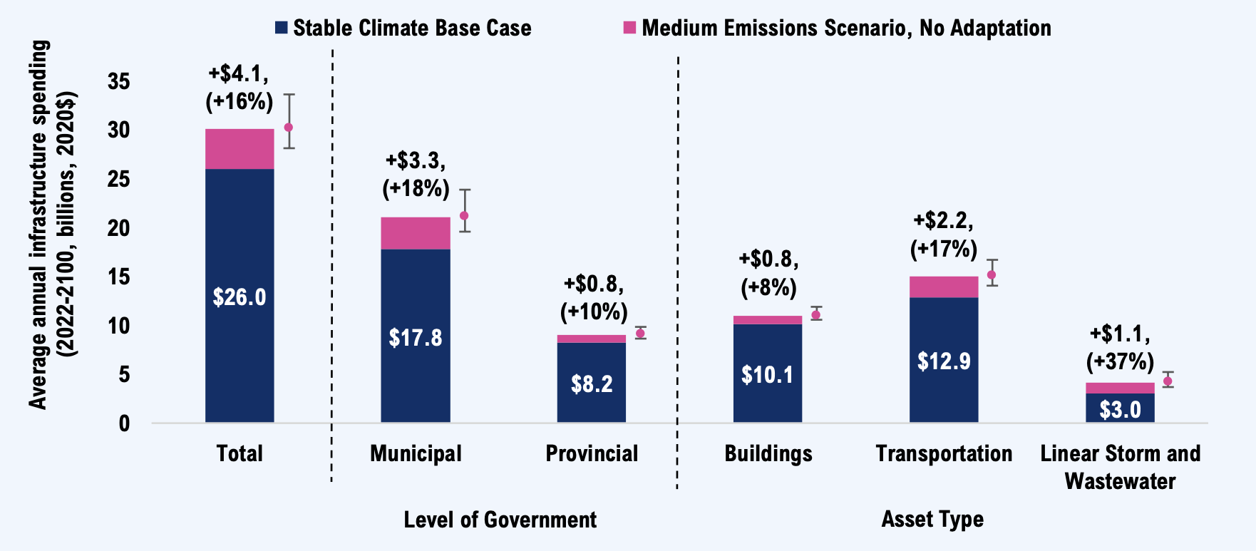
Note: Uncertainty bands represent the range of cost outcomes in the medium emissions scenario. see Accounting for uncertainty.
Source: FAO.
Ultimately, the extent of climate change will have a direct impact on the costs to maintain Ontario’s public infrastructure. In the absence of adaptation, the FAO estimates that Ontario’s public infrastructure costs will rise by approximately eight per cent (or about $2.0 billion per year) on average over the rest of the century for each degree Celsius increase in the global mean surface temperature beyond the 0.5°C in the base case.
Adaptation can lower climate-related infrastructure costs
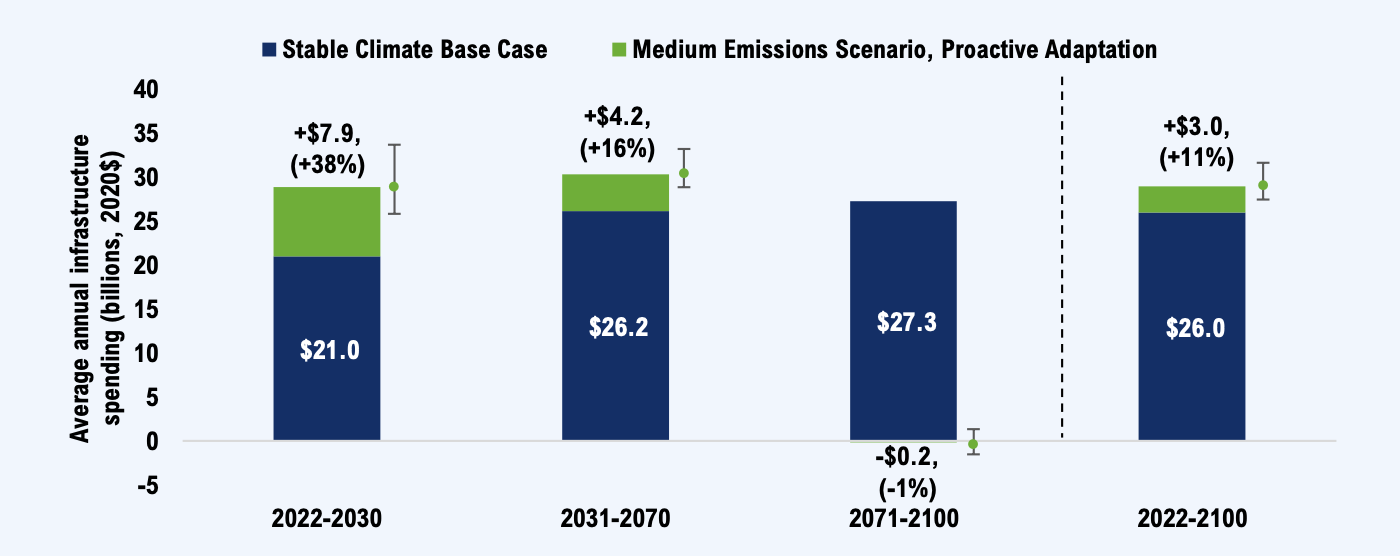
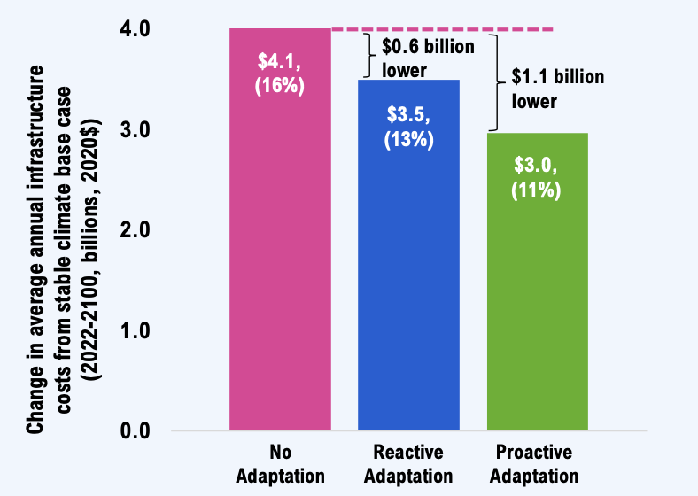
Figure 1‑2 Adaptation can lower infrastructure costs
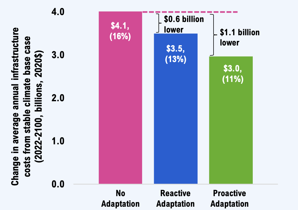
Note: Values represent the median projection of the medium emissions scenario. Uncertainty bands are omitted from this figure for clarity of presentation (see Accounting for uncertainty).
Source: FAO.
Adapting public infrastructure can help to avoid climate-related deterioration and operations and maintenance activities. However, adaptive actions can also raise public infrastructure costs. The FAO costed climate impacts to public infrastructure for multiple climate scenarios and across three asset management strategies. A no adaptation strategy assumes that public infrastructure is not adapted to withstand changing climate hazards. A proactive adaptation strategy assumes asset managers adapt infrastructure either during an asset’s next major rehabilitation or upcoming renewal, whichever comes first. A reactive adaptation strategy assumes infrastructure assets are adapted when replaced at the end of their useful lives.
The financial impact of extreme rainfall, extreme heat and freeze-thaw cycles will be material to the Province and municipalities regardless of which asset management strategy is pursued. However, the FAO estimates that on a constant dollar basis, average annual climate-related costs are highest under the no adaptation strategy ($4.1 billion per year, or 16 per cent above a stable climate base case) and lowest under the proactive adaptation strategy ($3.0 billion per year, or 11 per cent above a stable climate case case) in a medium emissions scenario. Across all climate scenarios, the proactive adaptation strategy carries the lowest climate-related costs in constant dollars.
Adaptation reduces the risk of climate-related infrastructure service disruption
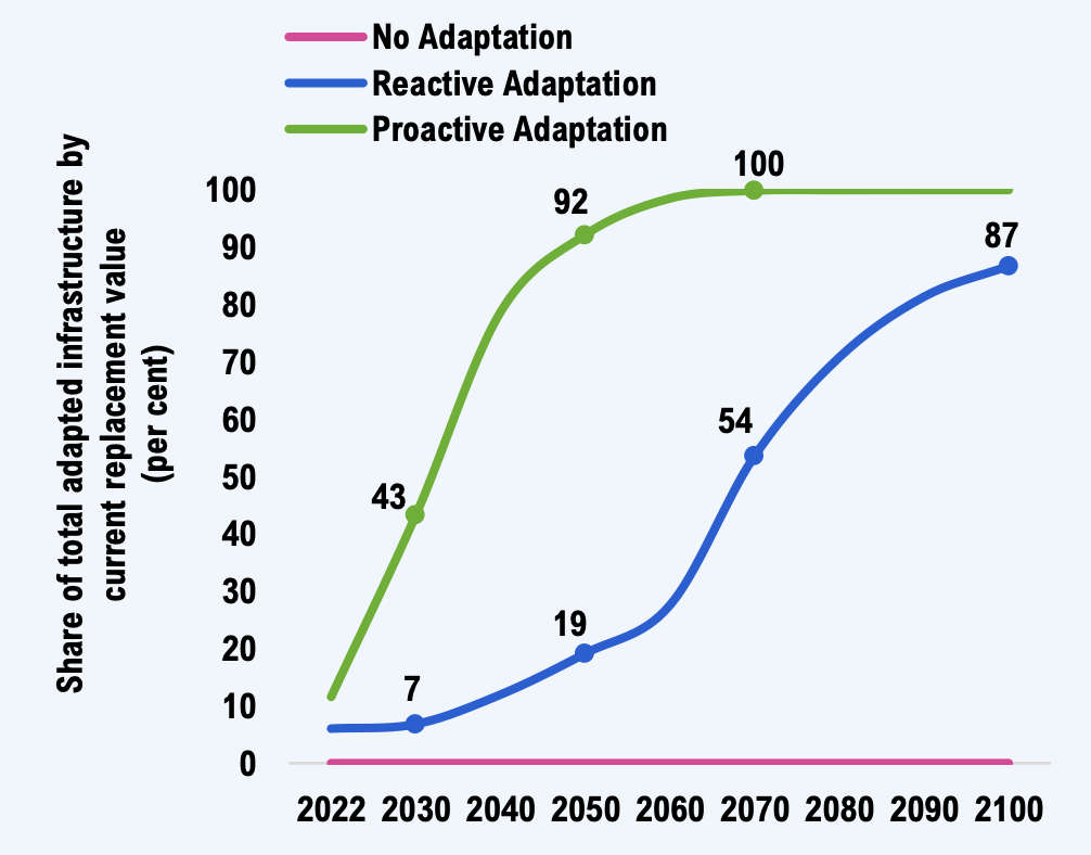
Adapting public infrastructure reduces its climate vulnerability and lowers the risk of infrastructure failure or loss of performance. The proactive adaptation strategy adapts all public infrastructure over the next five decades, rapidly improving the portfolio’s climate resilience. The reactive adaptation strategy adapts assets more slowly, leaving the majority of Ontario’s public infrastructure more vulnerable to climate risk though to the mid-2060s.
When public infrastructure suffers a loss of performance, or fails entirely, it can impose costs on households, businesses and the broader economy. For example, if extreme rainfall overwhelms stormwater infrastructure and the surrounding area floods, households and businesses may have to repair the flood damages. These broader societal costs are likely to be substantial but were beyond the scope of the FAO’s costing analysis.
The long-term budget impact of climate-related infrastructure costs for the provincial portfolio
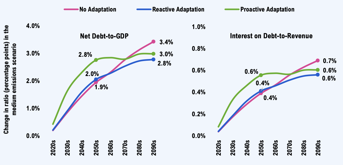
Figure 1‑4 Climate costs to provincial infrastructure are unlikely to significantly impact the Province’s long-term finances
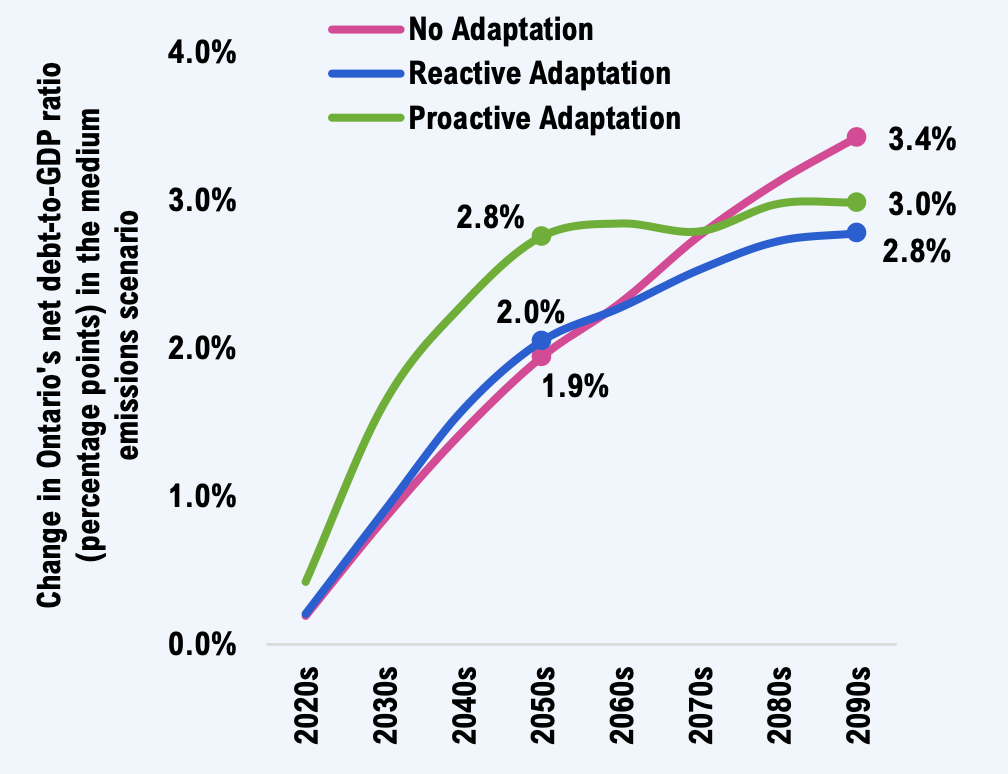
Note: Values represent the median projection of the medium emissions scenario. Uncertainty bands are omitted from this figure for clarity of presentation (see Accounting for uncertainty).
Source: FAO.
In a medium emissions scenario, climate-related infrastructure costs for the provincial portfolio would add 2.8 to 3.4 percentage points to the Province’s net debt-to-GDP ratio by the end of the century. For context, Ontario’s net debt rose from 10.4 per cent of GDP in 1981-82 to 38.3 per cent in 2022-23, an increase of 27.9 percentage points in 41 years. In the medium emissions scenario, the climate costs for provincial infrastructure are not likely to significantly impact the Province’s fiscal sustainability.
Early investment in the proactive strategy would minimize the risk of climate-related provincial infrastructure service disruption and would consume an additional 20 cents of every $100 dollars in revenue in the 2050s relative to the reactive strategy. However, by the 2090s, all asset management strategies have similar budgetary impacts.
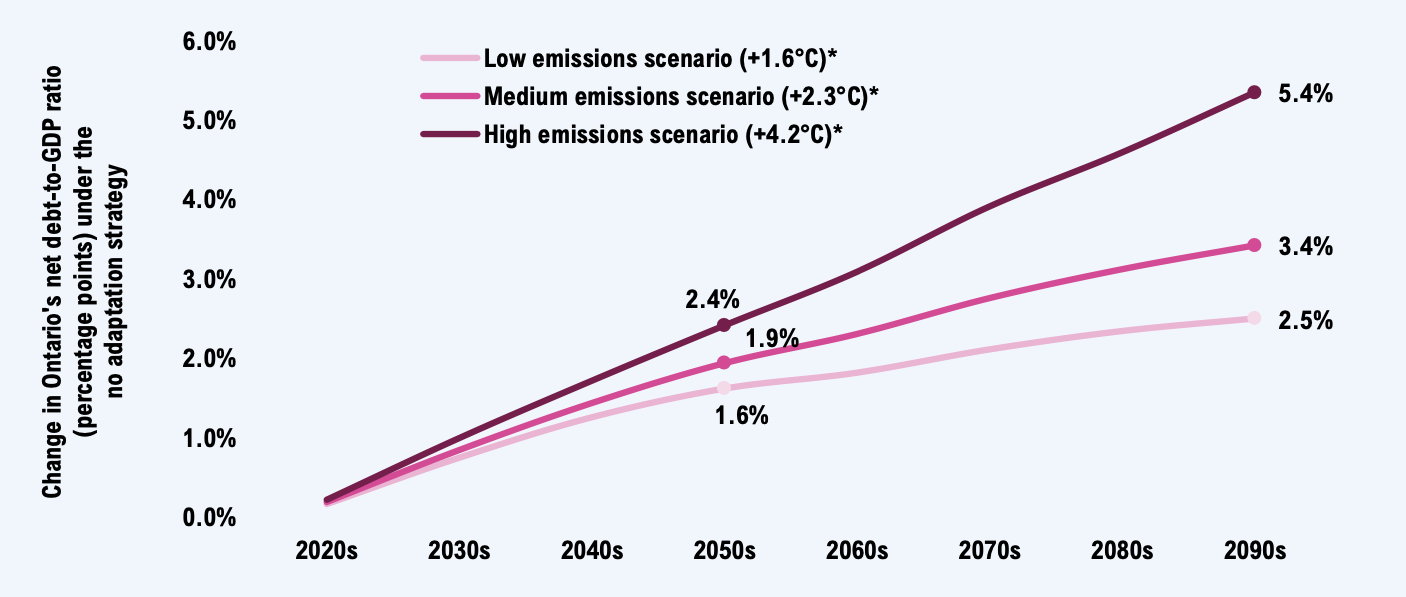
Climate scenarios with greater increases in global mean temperatures result in more significant fiscal outcomes due to more frequent and intense climate hazards. For example, in the absence of adaptation, the FAO estimates that Ontario’s net debt-to-GDP ratio would increase by 1.6 percentage points by the 2090s for every degree Celsius increase in global mean temperatures beyond 0.5ºC.
The impact of climate-related infrastructure costs for municipalities is projected to be four times larger than for the Province
Ontario’s 444 municipalities own 71 per cent ($506 billion) of the public infrastructure portfolio in the CIPI project’s scope. The municipal portfolio includes all the linear storm and wastewater infrastructure, which is more vulnerable to extreme rainfall than the other asset classes. As a result, Ontario’s municipalities are projected to incur about four times the climate-related infrastructure costs than the Province.
In the medium emissions scenario, municipal climate-related infrastructure costs are projected to range between $2.4 billion and $3.3 billion per year on average over the century, depending on the asset management strategy. These costs are equivalent to between five and seven per cent of total Ontario-wide municipal spending in 2020, similar to the amount municipalities spent on social housing, general government, or health and emergency services.
The impact of climate-related infrastructure costs for the combined provincial and municipal portfolios
To gauge the full magnitude of the CIPI project’s climate cost estimates, the FAO projected the impact of both provincial and municipal climate-related infrastructure costs on the Province’s long-term fiscal position. While the Province is not legally required to fund municipal financial liabilities, the intent of this analysis is to illustrate the size of the combined budgetary liability.
Figure 1‑5 Illustrative impact on provincial finances of climate costs for the entire provincial-municipal infrastructure portfolio
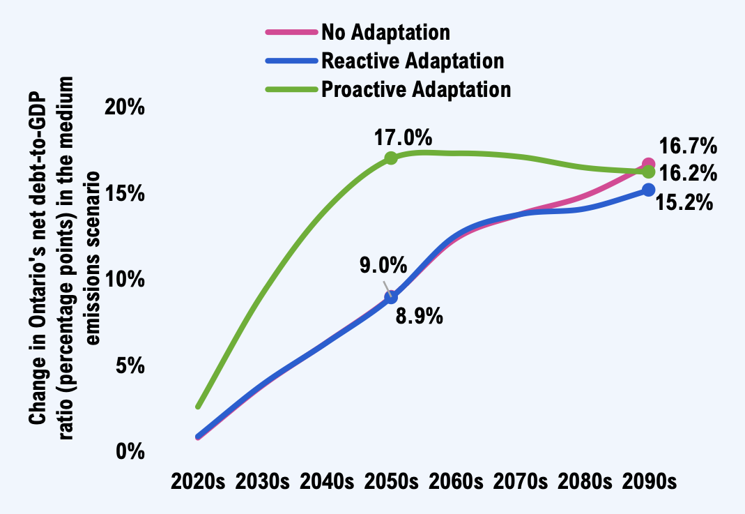
Note: Values represent the median projection of the medium emissions scenarioThe uncertainty bands are omitted from this figure for clarity of presentation (see Accounting for uncertainty).
Source: FAO.
Climate-related costs for the combined infrastructure portfolio would raise the Province’s net debt-to-GDP ratio by 15.2 to 16.7 percentage points by the 2090s in a medium emissions scenario. These impacts are much larger than for the provincial portfolio alone.
The fiscal impacts of the proactive strategy occur earlier in the century since investments are made to adapt roughly 90 per cent of provincial and municipal public infrastructure by 2050, versus roughly 20 per cent in the reactive strategy.
Early investments in the proactive strategy would minimize the risk of climate-related public infrastructure service disruption and would consume an additional $1.60 of every $100 dollars in revenue in the 2050s relative to the reactive strategy. However, all asset management strategies have similar budgetary impacts by the 2090s.
The Province’s climate change risk assessment aligns with CIPI
The Province recently released its Provincial Climate Change Impact Assessment (PCCIA), which found that “…all infrastructure across Ontario face climate risk.”[1] While the PCCIA examined a broader range of climate hazards on a different composition of public and private infrastructure asset classes, its conclusions on the climate vulnerability of public infrastructure are broadly aligned with those of the CIPI project.
The FAO’s climate costs are lower-bound estimates
Public infrastructure is one of many ways that climate change is impacting Ontario’s society and economy. Within the scope of climate change’s impact to public infrastructure, the FAO’s cost estimates reflect the lower bound of potential impacts. The CIPI project examined only three of many climate hazards, considered a subset of Ontario’s public infrastructure, and did not incorporate the broader costs to households and businesses of climate-related infrastructure service disruption.
2 | About the CIPI project
Canada has produced a growing body of work examining how climate change will impact public infrastructure. Recently, the Canadian government released its National Adaptation Strategy, which stated that there is a need to scale up investments to make public infrastructure more resilient to a changing climate.[2] Ontario also released its Provincial Climate Change Impact Assessment (PCCIA), which found that “…all infrastructure across Ontario face climate risk.”[3]
Despite numerous climate risk assessments, the cost implications of changing climate hazards for government infrastructure budgets remain largely unexplored, both in Canada and abroad. In response to this knowledge gap, a Member of Provincial Parliament asked the FAO to analyze the costs that the impacts of climate change could impose on Ontario’s provincial and municipal infrastructure, and how those costs could affect the long-term budget outlook of the Province. In response, the FAO launched its Costing Climate Change Impacts to Public Infrastructure (CIPI) project.
Given the complexity of the request, the CIPI project was carefully scoped in three important ways. First, despite the presence of many climate hazards, CIPI only considered three: extreme rainfall, extreme heat and freeze-thaw cycles. Second, while these three climate hazards will have a wide range of impacts on Ontario’s public infrastructure, CIPI included only 11 of the most important impacts on select asset classes. Third, only those costs borne by governments to maintain the current suite of infrastructure in a state of good repair were included. The broader societal costs to households and businesses from reductions or losses in infrastructure service provision were beyond the scope of the CIPI project.
The project began with two reports assessing the composition and state of repair of provincial and municipal infrastructure. Then, in the fall of 2021, the FAO released three reports: the CIPI project backgrounder, which described the overall context and methodology of the CIPI project; a report prepared by WSP Global, which detailed the engineering impacts of these climate hazards on public infrastructure; and the first CIPI sector report, which described how changes in these climate hazards will impact the long-term costs of maintaining Ontario’s public buildings and facilities in a state of good repair. This was followed by sector reports for transportation infrastructure and linear storm and wastewater infrastructure.
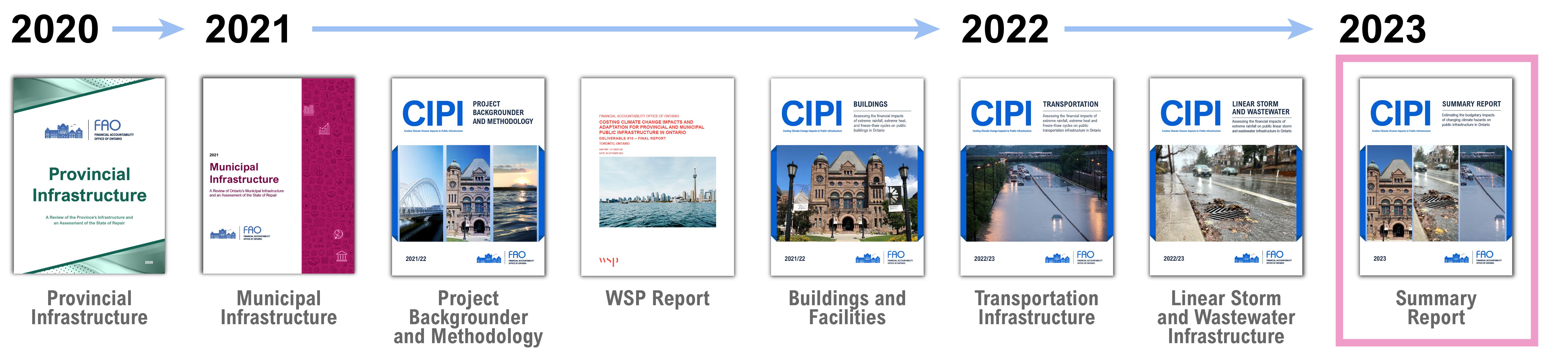
This summary report outlines the main results of the three sector reports and projects long-term budgetary impacts on key fiscal sustainability measures. In addition, WSP’s updated engineering assessment is available for download on the FAO’s website, as well as all historical and projected climate indicators used in the CIPI project. Municipal and region-specific results are available by request. All costs are expressed in 2020 constant dollars unless otherwise noted.
3 | Public infrastructure is vulnerable to changing climate hazards
Ontario has a large portfolio of public infrastructure
Figure 3‑1 The CIPI project examined $708 billion of provincial and municipal public infrastructure
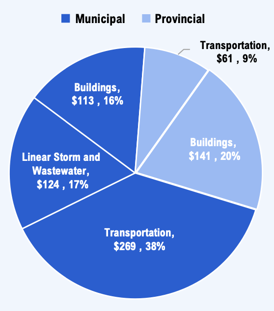
Note: CRV estimates are in real 2020 billion dollars. Percentage values refer to the share of total CRV.
Source: FAO.
The FAO’s Costing Climate Change Impacts to Public Infrastructure (CIPI) project focuses on $708 billion[4] (in current replacement value[5]) of provincial and municipally owned assets that encompassed three asset sectors: buildings, transportation infrastructure, and linear storm and wastewater infrastructure.[6]
- The buildings sector comprises buildings and facilities such as schools, hospitals, government administration buildings, social housing, water treatment plants, among others.
- Transportation infrastructure includes highways, arterials, collector roads, local roads, bridges, rail track and large structural culverts.
- Linear storm and wastewater infrastructure includes stormwater pipes, ditches and culverts, as well as wastewater sewers and sanitary force mains.
Ontario’s 444 municipalities own and manage $506 billion of this infrastructure, representing 71 per cent of the infrastructure assets in scope. The Province owns $202 billion, or 29 per cent of assets in scope. For context, the value of the portfolio under analysis is equivalent to almost three-quarters of Ontario’s 2021 economic output.
The project’s scope excludes federal infrastructure, infrastructure owned by Indigenous communities, linear potable water infrastructure, machinery and equipment assets, land, and infrastructure related to electricity generation, transmission and distribution.
While much of this portfolio was designed based on historical climate data, the climate is changing
To ensure safety and reliability, public infrastructure is designed, built and maintained to withstand a specific range of climate conditions typically based on historical climatic data. For example, Ontario’s Building Code uses climate design data based on historical weather observations, and Ontario’s Ministry of the Environment, Conservation and Parks requires municipalities to design sewers using historical precipitation data.[7] In addition, a survey of municipalities revealed that 57 per cent continue to rely on historical climate data when designing stormwater infrastructure.[8]
However, rising concentrations of greenhouse gases are increasing global mean temperatures, leading to more frequent and intense climate hazards in Ontario. The purpose of the CIPI project is to assess how future changes in climate variables will impact infrastructure costs relative to the recent past.
The historical baseline for CIPI is defined as the 1976-2005 period, as a significant portion of Ontario’s current public infrastructure was designed and built to the climate of that period. The “stable climate base case” assumes that all climate indicators remain at their 1976-2005 average levels. As the global mean surface temperature rose by 0.5ºC above pre-industrial averages by the 1976-2005 period, the stable climate base case incorporates 0.5ºC of global warming.[9] This stable climate base case cost projection will be compared in later chapters to projections that account for changing climate hazards, allowing the FAO to estimate the additional climate-related infrastructure costs.
While the global mean surface temperature has already risen substantially, the extent of future change will depend on the path of global greenhouse gas emissions. CIPI considered three possible global emissions scenarios based on the Intergovernmental Panel on Climate Change’s (IPCC) fifth comprehensive assessment. The low emissions scenario assumes a major and immediate turnaround in global climate policies. The medium emissions scenario assumes that global emissions peak in the 2040s, then decline rapidly thereafter. The high emissions scenario assumes global emissions continue to grow at their historical pace for most of the century.[10]
While the IPCC does not attach any likelihood to future emissions scenarios, further warming is projected to occur in all emissions scenarios.
Figure 3‑2 In all emissions scenarios, global temperatures are likely to rise by 1.5°C or more
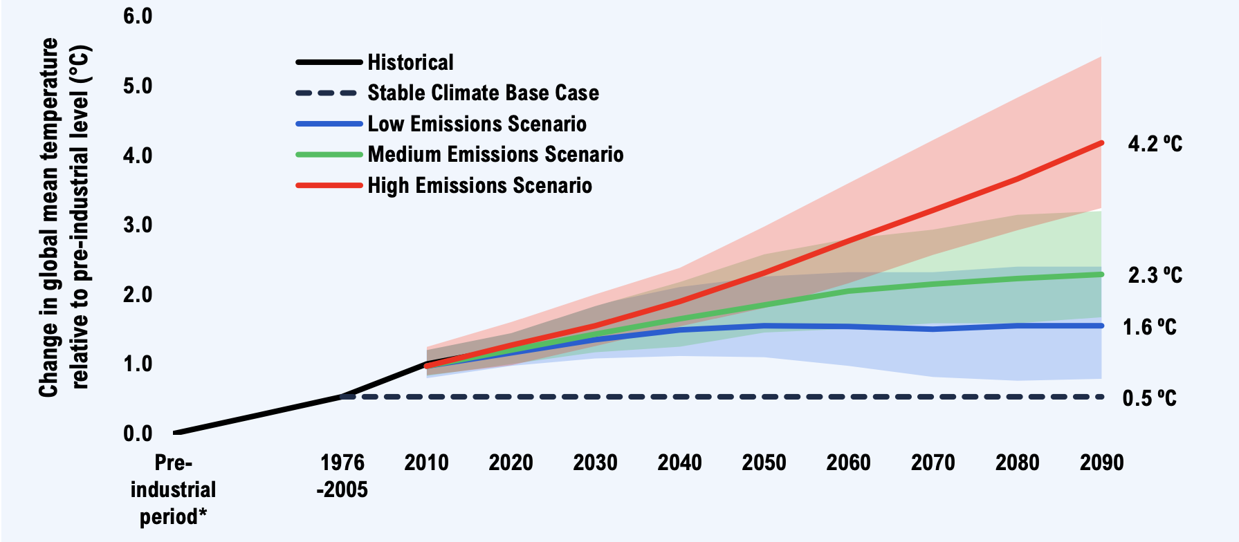
* Pre-industrial period represents average global temperatures over the 1850-1900 period.
Note: When different global climate models are given the same emissions path, they project slightly different global warming outcomes. The shaded areas show the possible range of warming outcomes in each emissions scenario, while the solid line shows the median model projection.
Source: Intergovernmental Panel on Climate Change, 2013, Table All. 7.5, page 1444, and FAO.
Climate change will bring more frequent and intense extreme heat and rainfall in Ontario, but fewer freeze-thaw cycles
Climate change is associated with many hazards to public infrastructure, which can take the form of extreme weather events or long-term chronic impacts. While public infrastructure faces many climate hazards,[11] CIPI focused on those that can be projected with reasonable scientific confidence, and which will have financially material impacts to public infrastructure budgets.
Working with WSP,[12] the FAO’s engineering consultant for the CIPI project, the scope of analysis was narrowed to three climate hazards that include extreme heat, extreme rainfall[13] and freeze-thaw cycles. Figure 3‑3 shows which of these three climate hazards were examined for each asset class.
Figure 3‑3 Scope of interactions between selected climate hazards and public asset classes
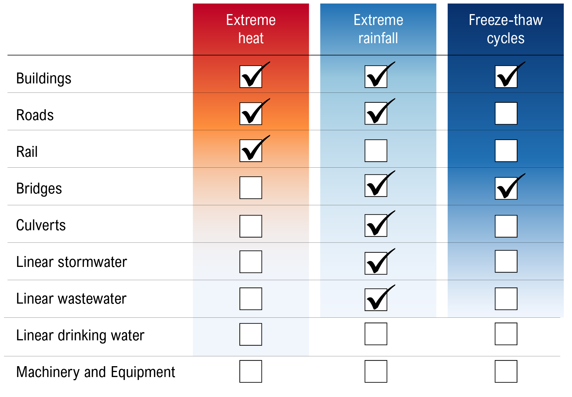
Source: WSP and FAO.
To acquire projections of key climate indicators for Ontario, the FAO partnered with the Canadian Centre for Climate Services (CCCS) at Environment and Climate Change Canada,[14] which provided projections for all climate variables used in the CIPI project.[15]
Over the rest of the 21st century, Ontario will experience more frequent and intense extreme heat, more frequent and intense extreme rainfall, and fewer freeze-thaw cycles on average across the province than occurred in the 1976-2005 base period. While the CIPI project used a broad range of climate variables to represent the climate hazards, Figure 3‑4 below shows how three select climate indicators representing these hazards are expected to change over the rest of the century.[16]
Figure 3‑4 On average, Ontario will experience more frequent and intense extreme heat and rainfall, and will have fewer freeze-thaw cycles
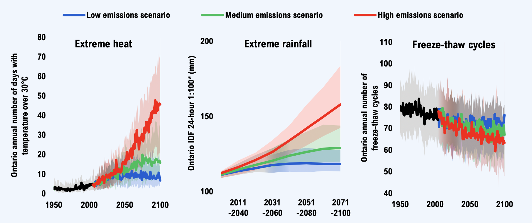
* This is the rainfall in millimetres that occurs in 24 hours for the 1-in-100-year storm event.
Note: Charts present Ontario average values. Regional projections vary.
Source: Canadian Centre for Climate Services. Click here to download the full dataset.
The annual number of “hot days” is one indicator of extreme heat, and occurs when the daily maximum temperature exceeds 30°C. On average across the province, hot days are expected to increase from 4 days per year in the 1976-2005 base period to 17 days (9 to 23 days)[17] by the late century period (i.e., 2071-2100) in the medium emissions scenario.
One indicator of extreme rainfall is the amount of rainfall that occurs in 24 hours for the 1-in-100-year storm event.[18] This storm event brought 103 mm of rain in a 24-hour period on average across the province in the 1976-2005 base period, which is projected to rise to 129 mm of rain (120 to 144 mm) by late century in the medium emissions scenario.
Freeze-thaw cycles (FTCs) are fluctuations between freezing and non-freezing temperatures that cause water to freeze (and expand) or melt (and contract). One indicator of FTCs is the annual number of days with daily maximum temperature above 0°C and daily minimum temperature below 0°C. In the medium emissions scenario, the number of annual freeze-thaw cycle events is expected to decline from 77 per year on average across the province in the 1976-2005 base period to an average of 68 (61 to 79) during the late century period.
These climate impacts will vary across the province as well as within regions. With the assistance of the CCCS, it was determined that providing climate change projections for 15 regions[19] in Ontario would adequately account for the expected geographic variability of climate change in Ontario. As an example, Figure 3‑5 shows the projected change in annual mean temperatures across the CIPI project’s regional breakdown.
Figure 3‑5 Northern Ontario is warming faster than southern regions
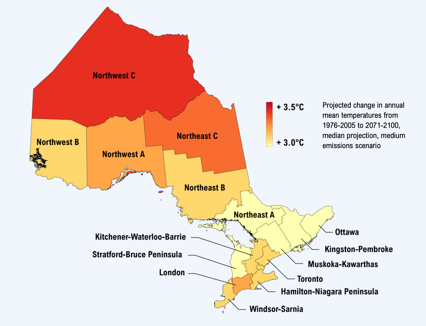
Source: Canadian Centre for Climate Services.
On average, Ontario is projected to warm faster than the global mean surface temperature, with Ontario’s north warming faster than its south.[20] As all asset locations in the CIPI portfolio are known, public infrastructure in each region was paired with the relevant climate impacts of that region to produce the costing results in the next chapter.
4 | Climate change will raise public infrastructure costs
Maintaining Ontario’s public infrastructure portfolio in a stable climate would cost $26 billion per year
Keeping public infrastructure in a state of good repair helps to maximize its benefits in the most cost-effective manner over time, and ensures these assets are operating in a condition that is considered acceptable from an engineering perspective. This requires annual spending on operations and maintenance (O&M) activities, as well as capital investments to intermittently rehabilitate assets or replace them at the end of their useful service lives. The capital investments and O&M spending required to maintain assets in a state of good repair are referred to as “infrastructure costs” throughout this report.
If the climate remained stable at 1976-2005 average levels, when much of the province’s infrastructure was designed and built, maintaining the $708 billion portfolio of existing public infrastructure would require an average of $26.0 billion per year (in 2020 constant dollars) in infrastructure costs over the rest of the century. In the next section, this stable climate cost projection will be compared to projections that account for changing climate hazards, allowing the FAO to estimate the additional climate-related infrastructure costs.
Figure 4‑1 Maintaining the $708 billion portfolio of provincial and municipal infrastructure in a stable climate would cost $26 billion per year
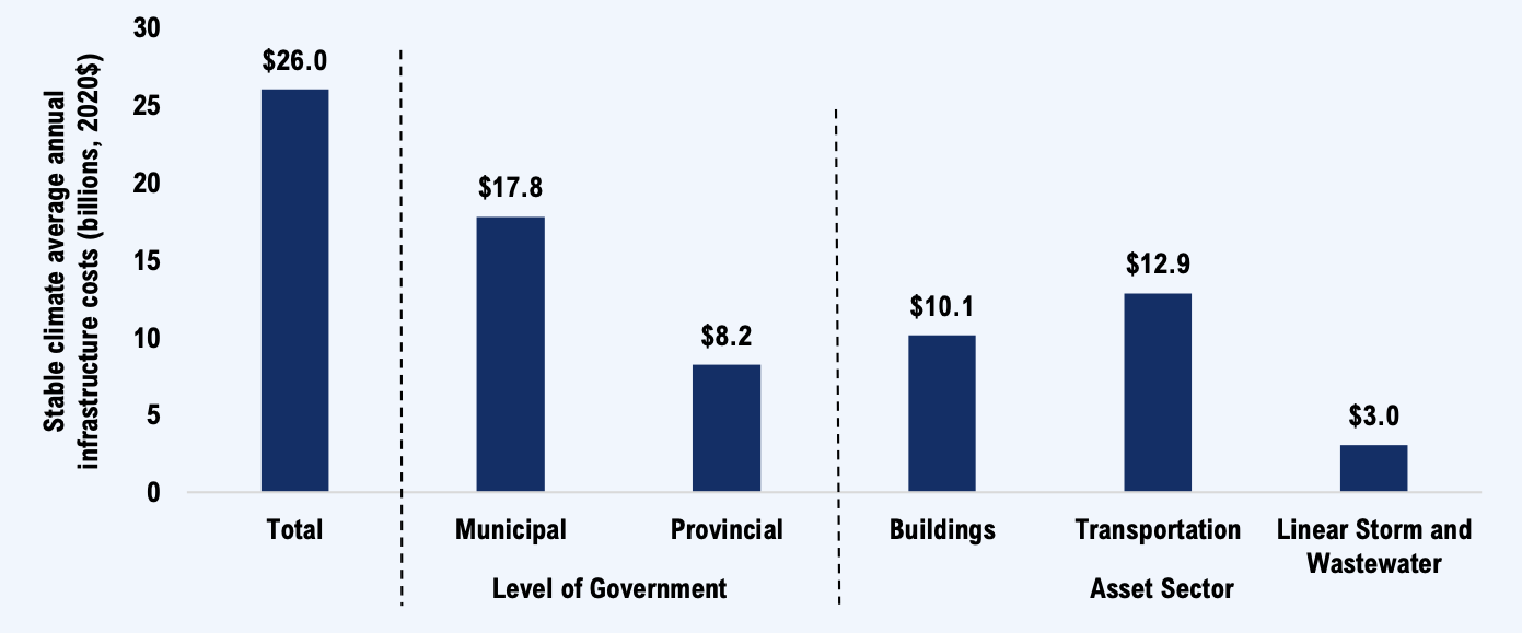
Note: The “stable climate base case” assumes that all climate indicators remain at their 1976-2005 average levels.
Source: FAO.
Ontario’s municipalities, which own almost three-quarters of this portfolio, would need to spend an average of $17.8 billion per year to maintain their assets in a state of good repair, while the Province would need to spend an average of $8.2 billion per year.
Infrastructure cost projections
The infrastructure cost projections presented throughout this report only relate to the existing $708 billion portfolio (as of 2020). They do not include the cost of assets either currently under construction, planned for future construction or necessary to meet future infrastructure demand. Cost projections assume that the funding required to address infrastructure repair backlogs and maintain a state of good repair is spent as necessary. In practice, not all infrastructure is maintained in a state of good repair and infrastructure backlogs exist.[21] To produce infrastructure cost projections for different climate scenarios, the FAO used a standard infrastructure deterioration model that was upgraded with “climate cost elasticities.” These climate cost relationships relate changes in climate variables to public infrastructure costs. WSP, FAO’s engineering consultant, provided these estimates. The full methodology is described in the WSP report and the CIPI backgrounder.[22]
Climate change will raise public infrastructure costs
Extreme heat and extreme rainfall have already become more frequent and intense relative to the late 20th century when a large portion of the province’s infrastructure was designed and built, while freeze-thaw cycles have become less frequent. Taken together, these changes are accelerating asset deterioration, resulting in the need for higher capital investments for more frequent rehabilitations and earlier renewals. In addition, changing climate hazards also require more operations and maintenance (O&M) activities, resulting in higher O&M spending. Figure 4‑2 provides select examples of how these changing climate hazards will impact public infrastructure.[23]
Figure 4‑2 Three examples of how climate hazards accelerate deterioration and raise operations and maintenance (O&M) costs
-
Buildings

Envelope*


Extreme high temperature fosters thermal expansion of materials and decreasing building performance. Freeze-thaw cycles cause envelope deterioration and cracking. Extreme rainfall results in erosion of porous materials, corrosion, and damage from leakage.
-
Transportation
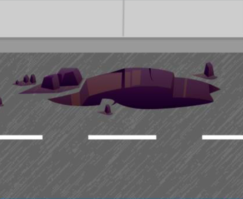
Roads
Extreme rainfall will increase erosion and washouts, while extreme heat will increase the risk of cracks forming through thermal weathering.
-
Linear Storm and Wastewater
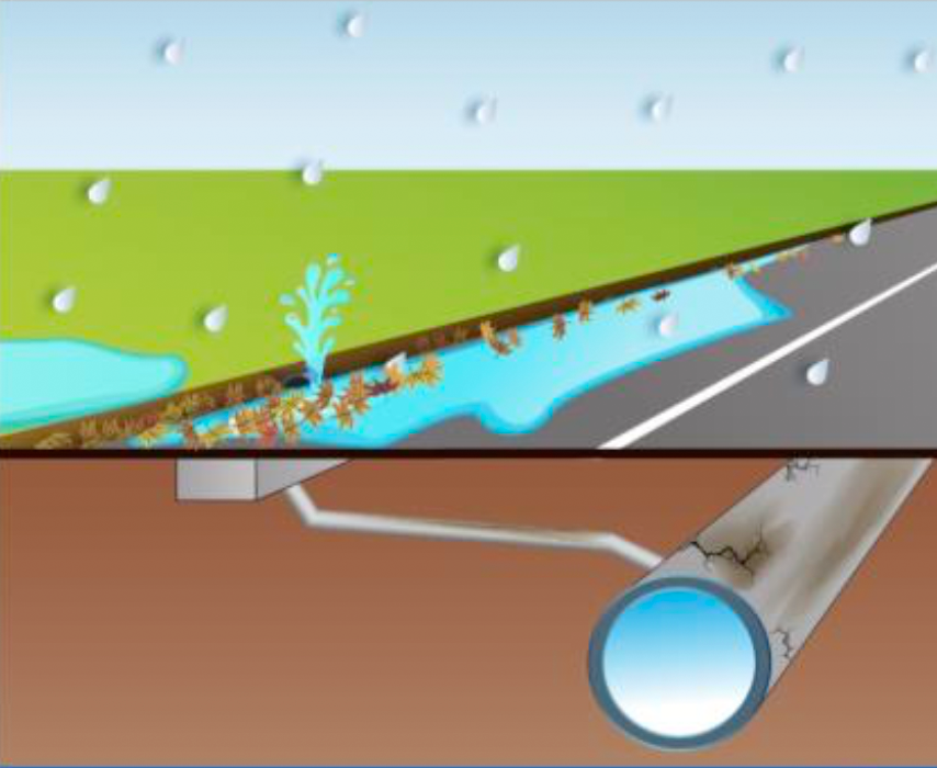
Stormwater - Pipe
More frequent and costly inspections and preventive maintenance required, as more debris, sediment and vegetation are expected to enter stormwater systems.
 Extreme Rainfall
 Extreme Heat
 Freeze-thaw Cycles
* Envelope represents a component of buildings, while roads and stormwater pipes represent specific assets.
Source: FAO and WSP.
While in practice many climate change adaptation initiatives are under way, to explore the cost implications of not adapting public infrastructure to changing climate hazards, the FAO developed a no adaptation asset management strategy. This strategy assumes that public infrastructure is not adapted to withstand changing climate hazards. Instead, asset managers pay the costs of climate-related accelerated deterioration and more frequent operations and maintenance activities.
Over the current decade (2022-2030), these climate-related impacts are projected to add an average of $2.6 billion ($1.4 to $4.4 billion)[24] per year to infrastructure costs. These climate-related costs would cumulate to $23 billion ($12 to $40 billion) by 2030 in the absence of adaptation.
Figure 4‑3 Climate-related costs will increase as hazards become more frequent and intense
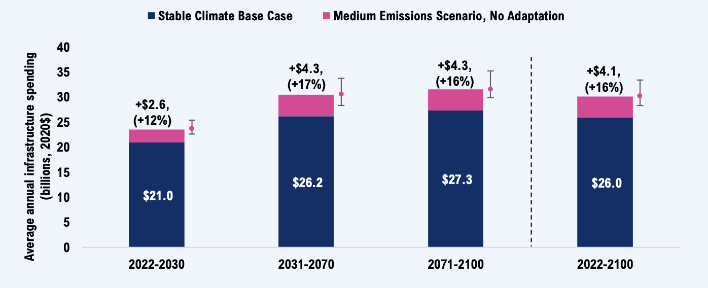
Note: Uncertainty bands represent the range of cost outcomes in the medium emissions scenario. see Accounting for uncertainty.
Source: FAO.
In the medium emissions scenario, climate-related costs increase through the mid-century period (2031-2070)[25] as extreme rainfall and extreme heat become more frequent and intense. Costs plateau in the late-century period (2071-2100) as the severity of these climate hazards levels off (see Figure 3‑4).
The estimated climate-related costs only account for the direct costs to governments of maintaining infrastructure in a state of good repair. They do not account for the broader societal costs to households and businesses from climate change’s impact on public infrastructure.[26] These broader climate-related costs are likely to be substantial but are beyond the scope of this analysis.
Accounting for uncertainty
The FAO’s cost projections account for three key types of uncertainty: emissions uncertainty, climate model uncertainty and infrastructure vulnerability uncertainty. Emissions uncertainty reflects the uncertain future path of global emissions and is represented by the three emissions scenarios – low, medium and high (see Figure 3‑2). For each global emissions scenario, different climate models project slightly different climate variable outcomes. This climate model uncertainty is represented by reporting the median (50th percentile) model projection, as well as the 10th and 90th percentile model projections of each emissions scenario. This produces nine climate scenarios.
In addition, the impact of a given change in climate hazard on infrastructure costs is also uncertain. In the absence of adaptation, infrastructure vulnerability uncertainty will depend on the design standards, age, condition, location and maintenance practices of individual assets. For adaptation costs, this uncertainty reflects the engineering options available to address specific climate hazards. The FAO commissioned an engineering survey to assess these climate vulnerabilities, which produced a range of opinion from “optimistic” to “pessimistic,” as well as the “most likely” climate vulnerability.[27] Incorporating these uncertainties into the nine climate scenarios produced 27 cost projections.
Figure 4‑4 The UN’s most likely warming outcomes align with the medium emissions scenario’s range
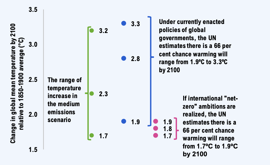
Source: Intergovernmental Panel on Climate Change, 2013, Table All.7.5, United Nations Environment Programme (2022) and FAO.
This report focuses on climate cost projections for the medium emissions scenario, whose global mean temperature projections closely align with those in a United Nation’s (UN) emissions assessment from October 2022.[28] The UN report estimates that under the current policies of global governments, and assuming no further emissions reductions are enacted, the global mean temperature has a 66 per cent chance of increasing by between 1.9 to 3.3°C by 2100 relative to the 1850-1900 pre-industrial period. If global “net zero” ambitions are realized by 2050, the UN estimates that global warming has a 66 per cent chance of staying below 1.7°C and 1.9°C by 2100.[29] Both of these outcomes are almost fully bounded by the range of warming in the medium emissions scenario (see Figure 3‑2).
Throughout this report, costs are presented as point estimates, which reflect the median (50th percentile) climate model projection combined with the “most likely” asset vulnerabilities. This is followed by a parenthesis showing the range of possible cost projections for the medium emissions scenario given the climate model and infrastructure vulnerability uncertainties. This range is bounded by the lower 10th percentile climate model projection combined with the “optimistic” asset vulnerabilities (the least costly outcome), and the upper 90th percentile climate model projection combined with the “pessimistic” asset vulnerabilities (the costliest outcome).
Global warming and the related climate cost outcomes could also occur outside of this range. These are presented selectively in this report as well as in the report’s Appendix.
Municipalities will bear most of the climate-related infrastructure costs
In the absence of adaptation, municipal infrastructure costs would increase by an average of $3.3 billion ($1.7 to $6.0 billion) per year over the century, while provincial costs would be expected to increase by $0.8 billion ($0.3 to $1.5 billion) per year. Municipalities bear most of the climate-related infrastructure costs estimated in the CIPI project in part because they own and manage over 70 per cent of the portfolio in scope (see Figure 3‑1), and because their asset portfolio is also more susceptible[30] to these changing climate hazards.
Figure 4‑5 Municipal infrastructure costs will rise more than provincial costs
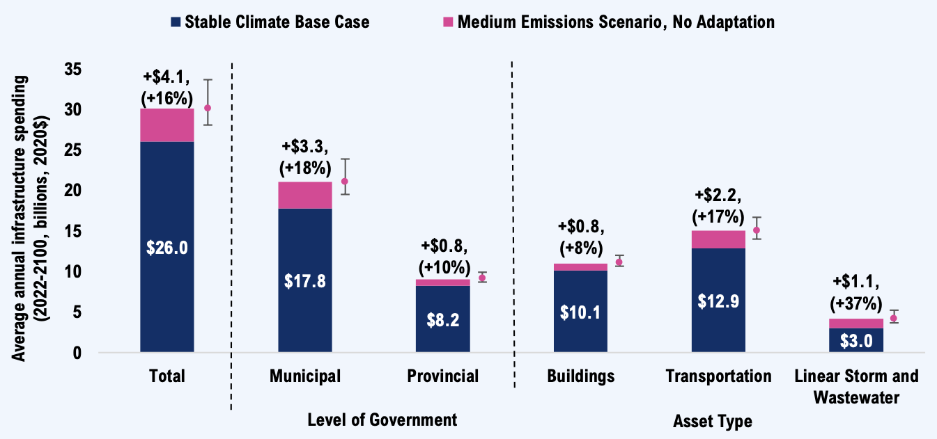
Note: Uncertainty bands represent the range of cost outcomes in the medium emissions scenario. see Accounting for uncertainty.
Source: FAO.
Under the no adaptation strategy, the infrastructure costs of public buildings would increase by 8 per cent (4 to 17 per cent). About 85 per cent of these additional climate-related costs are attributed to increased O&M activities, such as clearing of debris, inspections or increased HVAC use, while the remaining 15 per cent are due to capital investments associated with accelerated infrastructure deterioration, such as thermal expansion of the building envelope. The Province owns just over half of the public buildings in CIPI’s scope.
Transportation infrastructure costs would increase by 17 per cent (9 to 29 per cent). About two-thirds of the additional climate-related costs are due to increased O&M activities, such as more crack sealing, road patching, or bridge and culvert inspections, with the remaining one-third due to more rapid deterioration, such as increased scour and bridge erosions or transit track buckling. Municipalities own more than four times the amount of provincial transportation infrastructure by value in CIPI’s scope.
Linear storm and wastewater asset costs would increase by 37 per cent (19 to 69 per cent). The increased costs are almost entirely due to increases in O&M activities, such as more frequent and costly inspections, and preventive maintenance as more debris, sediment and vegetation are expected to enter storm and wastewater systems. These assets are owned exclusively by municipalities.
Public infrastructure costs could be much larger in the high emissions scenario
This chapter focused on costing results in the medium emissions scenario, where global emissions peak in the 2040s, and then decline rapidly thereafter. If global emissions follow the high emissions path, climate-related infrastructure costs in Ontario could be much larger. The range of potential cost increases in the higher emissions scenario is also much greater than the range of costs in the medium emissions scenario. Importantly, there is no likelihood attached to global emissions scenarios, or to the range of cost outcomes within each.
Figure 4‑6 Climate-related infrastructure costs could be much larger in the high emissions scenario
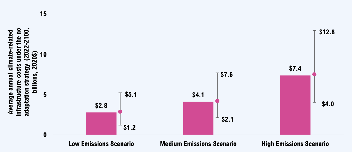
Note: Uncertainty bands represent the range of cost outcomes in each emissions scenario. see Accounting for uncertainty.
Source: FAO.
The profile of climate-related infrastructure costs over the century also differs significantly between the emissions scenarios. In the short term, climate-related costs are similar. By mid-century, costs in each emissions scenario begin to diverge, in line with the change in relative severity of climate hazards. By late century, costs diverge significantly. For example, the climate costs in the high emissions scenario are more than four times higher than in the low emissions scenario, and more than twice those in the medium emissions scenario.
Figure 4‑7 By late-century, climate-related infrastructure costs under the high emissions scenario are more than double those of the medium emissions scenario
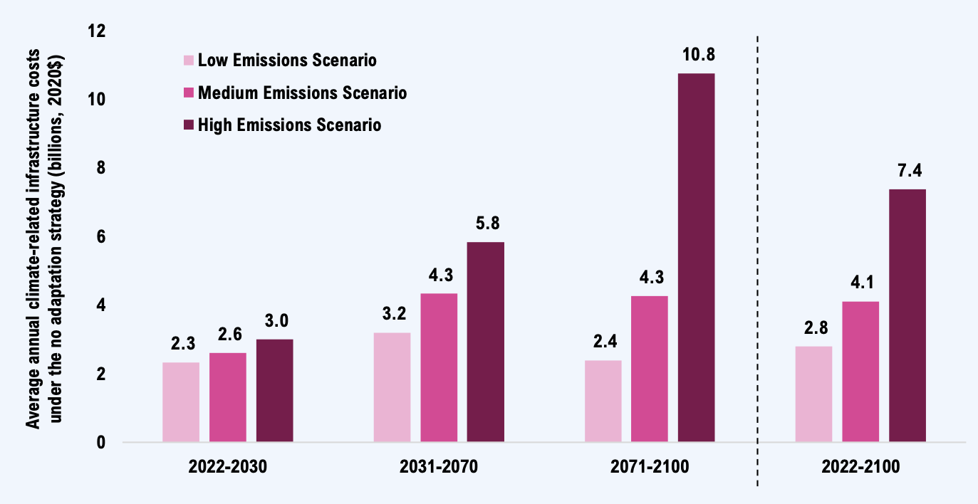
Note: Uncertainty bands are omitted for clarity. Values represent the median projection in each scenario. see Accounting for uncertainty.
Source: FAO.
Ultimately, the extent of increase in the global mean surface temperature will have a direct impact on the costs to maintain Ontario’s public infrastructure. Across all climate scenarios, and in the absence of adaptation, the FAO estimates that public infrastructure costs will rise by approximately eight per cent (or roughly $2.0 billion per year) on average over the rest of the century for each degree Celsius increase in global mean surface temperatures beyond 0.5°C.
5 | Adaptation can lower climate related infrastructure costs
Public infrastructure can be adapted to withstand more frequent and intense climate hazards
The previous chapter outlined the climate-related costs to public infrastructure in the absence of adaptation actions. Adapting public infrastructure can help avoid the accelerated deterioration and increased O&M activities associated with more frequent and intense climate hazards. Adaptation can take many forms. Figure 5‑1 provides three examples.[31]
Figure 5‑1 Adapting infrastructure to withstand changing climate hazards can take many forms
-
Buildings

Envelope*
Finishes on the exterior need to be more sustainable to withstand heat and maintain the thermal protection of the indoor environment, shielding other building components from much of the stress of extreme heat events.
Roof drainage needs to be sized for future rainfall projections and sufficiently graded to limit ponding. -
Transportation

Roads
Using a higher temperature grade asphalt binder can help reduce the risk of permanent deformation from extreme heat.
Mitigative measures against warping / curling and blow-up due to slab expansion include shortening joint spacing and installing high-quality expansion joints.
Specialized asphalt mixes and higher quality materials can mitigate drainage or erosion issues caused by extreme rainfall. -
Linear Storm and Wastewater
Stormwater - Pipe
Incorporate source control measures and green infrastructure solutions to soak rain into the ground and reduce runoff. Upsize pipes if necessary and ensure downstream stormwater systems can accommodate the higher flows.
* Envelope represents a component of buildings, while roads and stormwater pipes represent specific assets.
Source: FAO and WSP.
To assess the cost impacts of adapting public infrastructure, the FAO developed two representative adaptation strategies, where the speed of adaptation differs in each strategy.
- Proactive adaptation – asset managers adapt infrastructure either during an asset’s next major rehabilitation or upcoming renewal, whichever comes first. This strategy fully adapts the infrastructure portfolio by 2070.
- Reactive adaptation – asset managers adapt infrastructure assets only when they are replaced at the end of their useful lives. This strategy results in a slower pace of adaptation compared to the proactive strategy. By the end of the century, just under 90 per cent of assets are adapted.
Public infrastructure assets will continue to incur accelerated deterioration and require increased O&M activities from more frequent and intense climate hazards (as in the no adaptation strategy) until asset managers adapt their infrastructure. Once adapted, assets are assumed to be resilient to these climate hazards and avoid these climate-related infrastructure costs.
Adaptation will increase the costs to maintain infrastructure
If a proactive adaptation strategy is pursued, infrastructure costs would increase significantly in the short term, as substantial capital investments would be required to adapt almost half of the infrastructure portfolio by 2030. Over the 2022-2030 period, climate-related infrastructure costs under the proactive adaptation strategy average $7.9 billion ($4.8 to $12.6 billion), cumulating to $71 billion ($44 to $113 billion) by 2030 in the medium emissions scenario.
Figure 5‑2 Proactive adaptation requires significant upfront spending
Note: Uncertainty bands represent the range of cost outcomes in the medium emissions scenario. see Accounting for uncertainty. The proactive adaptation strategy assumes that infrastructure is adapted at the first available opportunity, and that the portfolio is fully adapted by 2070.
Source: FAO.
In the mid-century period, the pace of adaptation slows, resulting in an average of $4.2 billion ($2.6 to $6.9 billion) per year in additional climate-related costs. By late century, all assets are adapted, and infrastructure costs fall slightly below the stable climate base case as fewer infrastructure renewals occur during this period relative to the stable climate base case.[32]
If a reactive adaptation strategy is pursued, infrastructure costs would also increase in the short term but at a slower pace than under the proactive adaptation strategy. Over the 2022-2030 period, climate-related infrastructure costs under the reactive adaptation strategy average $3.1 billion ($1.6 to $5.3 billion) per year, cumulating to $28 billion ($15 to $48 billion) by 2030 in the medium emissions scenario.
In the mid-century period, as the pace of adaptation increases and extreme rainfall and heat become more frequent and intense, average climate-related costs increase to $4.4 billion ($2.0 to $8.1 billion) per year. By late century, as most assets are adapted, climate-related infrastructure costs average $2.4 billion ($1.5 to $4.5 billion) per year.
Figure 5‑3 Slower pace of adaptation under the reactive strategy results in a more gradual increase in costs
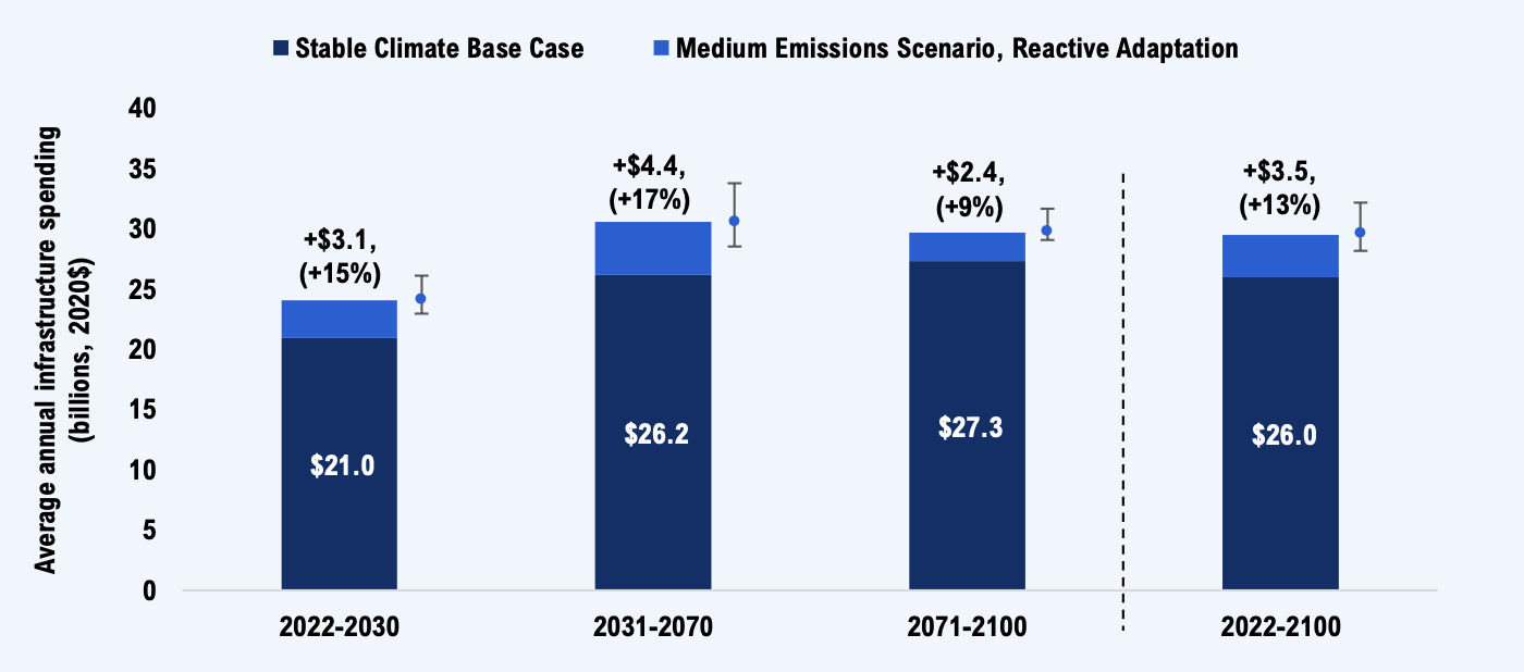
Note: Uncertainty bands represent the range of cost outcomes in the medium emissions scenario. see Accounting for uncertainty. The reactive adaptation strategy assumes that infrastructure assets are adapted when they are replaced at the end of their useful lives, and that half the portfolio is adapted by 2070 and 90 per cent by 2100.
Source: FAO.
Adaptation reduces the climate vulnerability of public infrastructure
Adapting public infrastructure reduces its climate vulnerability and lowers the risk of infrastructure failure or loss of performance. The quicker assets are adapted, the greater the reduction of climate risk. Figure 5‑4 shows the share of assets adapted (by CRV) over the projection under each of the asset management strategies.
Figure 5‑4 Proactive adaptation strategy sees all assets adapted to changing climate hazards by 2070
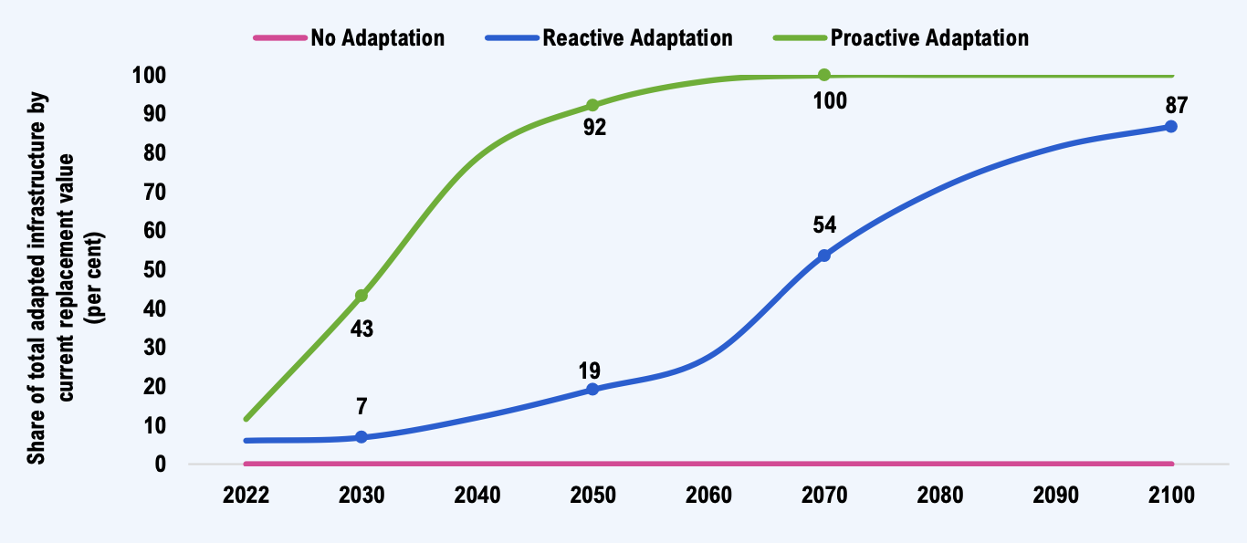
Source: FAO.
The proactive adaptation strategy sees 43 per cent of the portfolio adapted by 2030, 92 per cent by 2050 and 100 per cent by 2070. This strategy most rapidly lowers the climate vulnerability of Ontario’s public infrastructure. The reactive adaptation strategy undertakes adaptation more slowly, has lower upfront spending than the proactive strategy, but leaves the majority of Ontario’s public infrastructure more vulnerable to climate risk though to the mid-2060s. Even by the end of the century, the reactive strategy leaves over 10 per cent of public infrastructure exposed to more frequent and intense climate hazards. The no adaptation strategy carries the highest climate risk since no assets are adapted over the projection.
When public infrastructure suffers a loss of performance, or fails entirely, it can impose costs on households, businesses and the broader economy. For example, if extreme rainfall overwhelms stormwater infrastructure and the surrounding area floods, households and businesses may have to repair the flood damages. While these broader societal costs are likely to be substantial, they are not incorporated in the FAO’s costing analysis, which only includes the costs incurred to provincial and municipal infrastructure budgets.
Adaptation strategies result in lower average annual infrastructure costs
The financial impact of extreme rainfall, extreme heat and freeze-thaw cycles will be material to the Province and municipalities regardless of which asset management strategy is pursued. However, the FAO estimates that on a constant dollar basis, average annual climate-related costs are highest under the no adaptation strategy and lowest under the proactive adaptation strategy.
Figure 5-5 compares the climate-related infrastructure costs of all three asset management strategies in the medium emissions scenario. The proactive adaptation strategy results in the smallest increase in average annual infrastructure costs over the century at $3.0 billion per year. These climate-related costs represent an 11 per cent increase in infrastructure costs above the stable climate base case and are $1.1 billion lower per year on average than the no adaptation strategy.
Figure 5‑5 Adaptation can lower infrastructure costs
Note: Results presented are for the medium emissions scenario. The uncertainty bands are omitted from this figure for clarity of presentation (see Accounting for uncertainty). The Results Appendix contains the full range of costs in each asset management strategy. Adaptation strategies are defined here.
Source: FAO.
As the direct infrastructure costs to governments are included in each strategy but the societal costs of infrastructure service disruptions are not, these results reflect the impact on government budgets and should not be interpreted as a society-wide cost-benefit analysis.
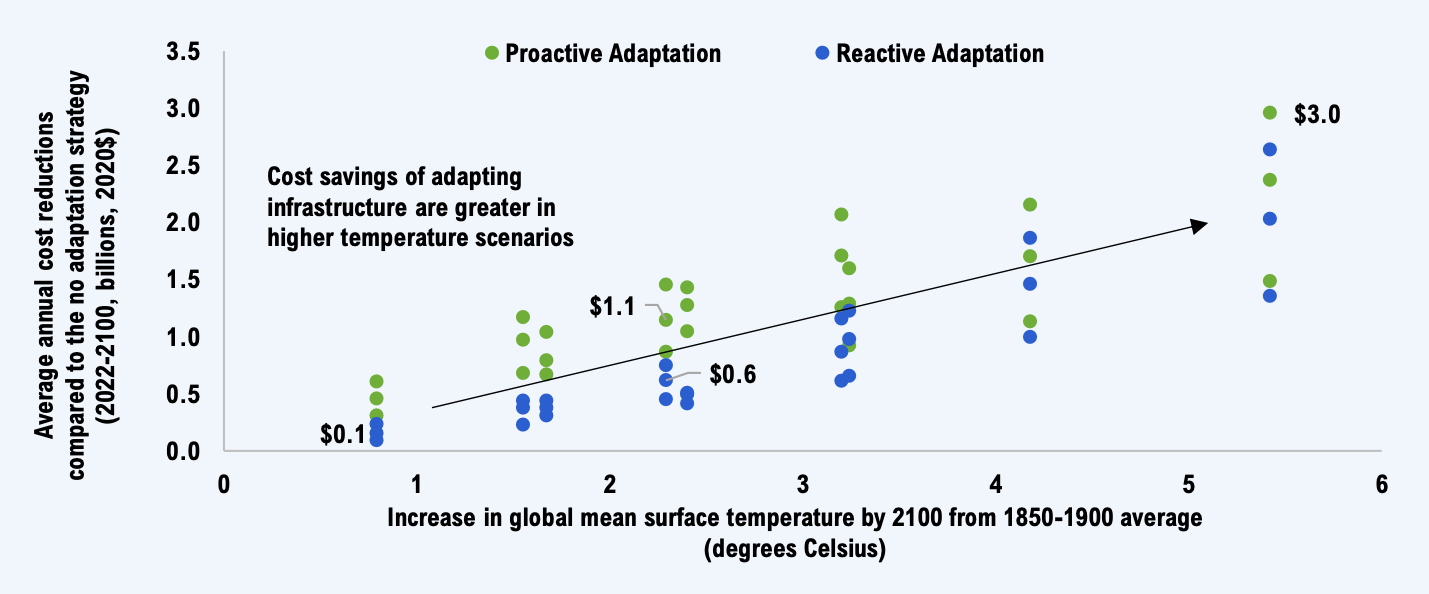
Across all climate scenarios, adaptation strategies are consistently less expensive over the century when compared with the no adaptation strategy, with the proactive strategy consistently the least expensive. Figure 5‑6 shows adaptation cost savings for the full range of potential global mean temperature increases. Each dot represents the average annual cost savings of adaptation relative to not adapting for a specific combination of climate scenario and asset vulnerability.
Cost savings of adapting infrastructure are larger in higher temperature scenarios, due to the avoidance of infrastructure damage and higher O&M costs from more severe climate hazards.
Figure 5‑6 Cost savings of adaptation strategies are greater in scenarios with higher global mean temperatures
Note: Each dot is a specific cost projection comprised of a combination of three emissions scenarios, three climate projections in each emissions scenario, and three assumptions for infrastructure vulnerability. see Accounting for uncertainty.
Source: FAO.
In the next chapter, the climate-related infrastructure costs are incorporated into the FAO’s long-term fiscal projections, which include the interest costs associated with borrowing to fund capital investments and higher climate-related operating expenses.
6 | Climate-related infrastructure costs will impact government budgets
The long-term budget impact of climate-related infrastructure costs for the provincial portfolio
To assess the impact of higher climate-related infrastructure costs on Ontario’s finances over the long term, the FAO focused on the effect that these climate-related infrastructure costs could have on two key metrics: the Province’s net debt-to-GDP ratio and the interest on debt-to-revenue ratio.
- Net debt as a share of GDP is an indicator of the government’s ability to service its debt obligations. A significant and prolonged deterioration in this indicator over time could raise concerns about the government’s ability to deliver on its budgetary responsibilities.
- Interest on debt as a share of revenue is a measure of budgetary flexibility. Higher interest payments as a share of revenue indicate that the government has a smaller share of revenue available to spend on key programs such as health care or education.[33]
Focusing on the provincially owned portion of Ontario’s infrastructure portfolio, Figure 6‑1 shows how climate-related infrastructure costs would impact these two measures of provincial budgetary health. Overall, in the medium emissions scenario, the climate costs to provincial infrastructure are not likely to significantly impact the Province’s fiscal sustainability under any of the asset management strategies.
Climate-related infrastructure costs result in higher spending, more borrowing and higher interest costs relative to the stable climate base case.[34] These costs are projected to raise the Province’s net debt-to-GDP ratio by 2.8 to 3.4 percentage points by the 2090s, and increase Ontario’s interest on debt-to-revenue ratio by between 0.6 and 0.7 percentage points in the medium emissions scenario. For context, Ontario’s net debt rose from 10.4 per cent of GDP in 1981-82 to 38.3 per cent in 2022-23, an increase of 27.9 percentage points in 41 years, and Ontario’s debt-interest payments consumed 6.0 per cent of total revenue in 1981-82, which rose to 15.5 per cent of revenue in 1999-00 before declining to 6.4 per cent in 2022-23.
Figure 6‑1 Climate costs to provincial infrastructure are unlikely to significantly impact the Province’s long-term finances
Note: The uncertainty bands are omitted from this figure for clarity of presentation (see Accounting for uncertainty). Values represent the median projection of the medium emissions scenario. Adaptation strategies are defined here. The Results Appendix contains the full range of fiscal results for the three asset management strategies.
Source: FAO.
All asset management strategies have similar budgetary impacts by the 2090s. The fiscal impacts of the proactive adaptation strategy occur earlier since investments are made to adapt about 90 per cent of provincial public infrastructure by 2050, compared to 20 per cent under the reactive adaptation strategy (see Figure 5‑4). Early investments under the proactive adaptation strategy would minimize the climate risk of provincial infrastructure service disruption and would consume an additional 20 cents of every $100 dollars in revenue in the 2050s relative to the reactive adaptation strategy.
Higher global temperatures would increase the climate-related impact to provincial finances
Greater increases in global mean temperatures result in more significant fiscal outcomes due to more frequent and extreme climate hazards and higher climate-related infrastructure costs, regardless of the asset management strategy undertaken. Figure 6‑2 shows the impact to the Province’s net debt-to-GDP ratio of the no adaptation strategy in the low, medium and high emissions scenarios. In the absence of adaptation, the FAO estimates that Ontario’s net debt-to-GDP ratio would increase by 1.6 percentage points by the 2090s for every degree Celsius increase in global mean temperatures beyond 0.5ºC.
Figure 6‑2 Higher global temperatures would raise climate-related infrastructure costs and the Province’s net debt-to-GDP ratio
* The increase in global mean surface temperatures by 2100 relative to the 1850-1900 average.
Note: The uncertainty bands are omitted from this figure for clarity of presentation (see Accounting for uncertainty). Values represent the median projection in each emissions scenario. See the Results Appendix for full range of fiscal outcomes.
Source: FAO.
Building new assets will increase the fiscal impact of these climate hazards
The CIPI project focused on the impact of climate hazards on existing infrastructure. However, as the population grows, new public infrastructure assets will be built. These new assets will also be impacted by the changing climate, as will the costs to build and maintain them. If expansionary assets were incorporated into the FAO’s analysis, the climate-related costs to maintain infrastructure would increase, further raising the fiscal impacts shown above for all asset management strategies.
The impact of climate-related infrastructure costs on municipalities is projected to be four times larger than for the Province
Ontario’s 444 municipalities own 71 per cent of the portfolio of public infrastructure in the CIPI project’s scope. In addition, their portfolio includes all the linear storm and wastewater infrastructure, which is much more vulnerable to extreme rainfall than the other asset classes. As a result, Ontario’s municipalities are projected to incur about four times the climate-related infrastructure costs than the Province.
In the medium emissions scenario, municipal climate-related infrastructure costs are projected to range between $2.4 billion to $3.3 billion per year on average over the century, depending on the asset management strategy. These costs are equivalent to between five per cent and seven per cent of total municipal spending in 2020, similar to the amount municipalities spent on social housing, general government, or health and emergency services.
Figure 6‑3 Climate-related costs will be equivalent to municipal spending on social housing, general government, or health and emergency services in the medium emissions scenario
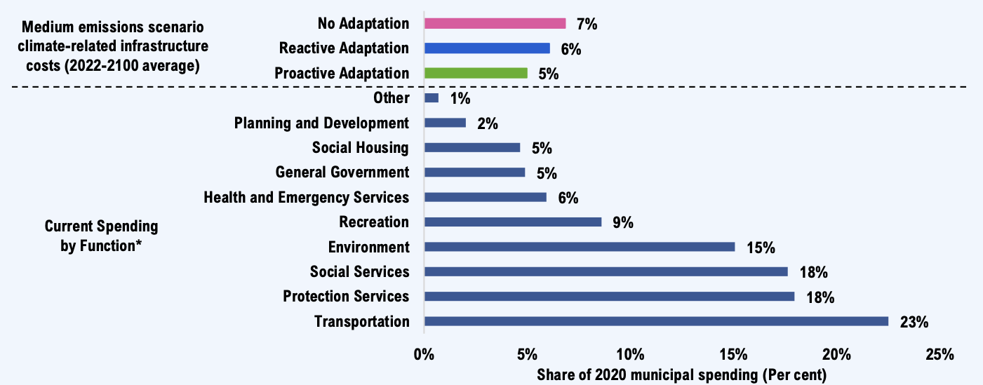
* Municipal spending in 2020 totalled $47.9 billion.
Note: Climate-related costs omit uncertainty bands from this figure for clarity of presentation (see Accounting for uncertainty). Values represent the median projection of the medium emissions scenario.
Source: Financial Information Return and FAO.
The proactive adaptation strategy results in the lowest average infrastructure costs over the projection. In addition, the proactive adaptation strategy would minimize the climate risk of public infrastructure service disruption and failure relative to the other strategies. However, the proactive adaptation strategy would require significant upfront investment, worth about 14 per cent of current municipal spending over the current decade to adapt about 43 per cent of municipal infrastructure assets. These rapid investments would enable the municipal infrastructure portfolio to avoid the accelerated deterioration and higher O&M costs seen under the other strategies in later decades, particularly in the 2071-2100 period.
Figure 6‑4 Proactive adaptation would require significant upfront spending
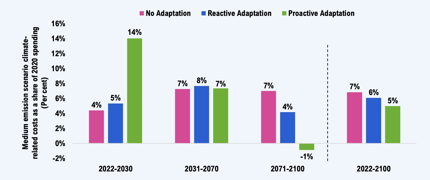
Note: The uncertainty bands are omitted from this figure for clarity of presentation (see Accounting for uncertainty). Values represent the median projection of the medium emissions scenario.
Source: Financial Information Return and FAO.
The impact of climate-related infrastructure costs for the combined provincial and municipal portfolios
To gauge the full magnitude of the CIPI project’s climate cost estimates, the FAO projected the impact of both provincial and municipal climate-related infrastructure costs on the Province’s long-term fiscal position. While the Province is not legally required to fund municipal financial liabilities, the intent of this analysis is to illustrate the size of the combined budgetary liability.
Figure 6‑5 shows the fiscal impact of climate-related costs on the Province’s finances for the combined provincial and municipal portfolio in the medium emissions scenario. Given the much larger size of the combined infrastructure portfolio, the impacts are much larger than for the provincial portfolio alone.
Climate costs for the combined infrastructure portfolio would raise the Province’s net debt-to-GDP ratio by 15.2 to 16.7 percentage points by the 2090s, and increase Ontario’s interest on debt-to-revenue ratio by between 3.1 and 3.4 percentage points, in the medium emissions scenario.
Figure 6‑5 Illustrative impacts on Provincial finances from climate costs to the entire provincial-municipal infrastructure portfolio
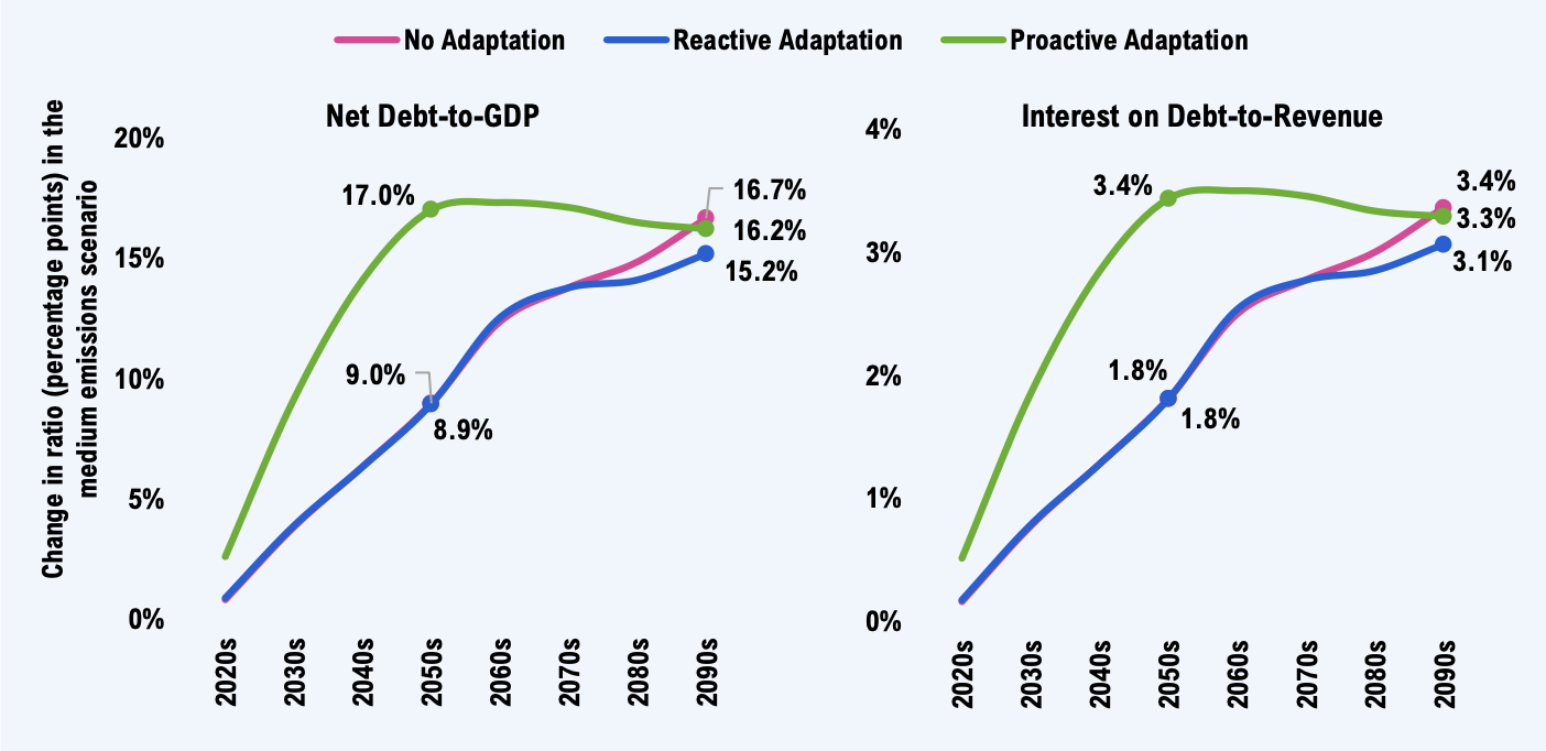
Note: The uncertainty bands are omitted from this figure for clarity of presentation (see Accounting for uncertainty). Values represent the median projection of the medium emissions scenario. The Results Appendix contains the full fiscal results for the three asset management strategies. Adaptation strategies are defined here.
Source: FAO.
All asset management strategies have similar budgetary impacts by the 2090s. The fiscal impacts of the proactive adaptation strategy occur earlier in the century since investments are made to adapt about 90 per cent of provincial and municipal public infrastructure by 2050, compared to 20 per cent under the reactive strategy (see Figure 5‑4). Early investment under the proactive adaptation strategy would minimize the climate risk of the entire provincial and municipal infrastructure portfolio and would consume an additional $1.60 of every $100 dollars in provincial revenue in the 2050s relative to the reactive adaptation strategy.
7 | The Province’s climate risk assessment aligns with CIPI
In August 2023, the government released its Provincial Climate Change Impact Assessment (PCCIA). The purpose of the assessment was to “…help government and public and private institutions better understand where and how climate change is likely to affect communities, critical infrastructure, economies and the natural environment so we can make more informed decisions on planning and investments to keep our communities healthy and safe.”[35]
The PCCIA examined numerous climate hazards, concluding that: “…extreme heat, extreme precipitation and seasonal temperature-related impacts are the drivers of highest risks across Ontario.”[36] The PCCIA examined climate risks in five areas of focus, including infrastructure. On infrastructure, the PCCIA noted that:
This impact assessment finds that all infrastructure across Ontario face climate risk. In fact, not a single asset included in this assessment is considered to have a risk less than ‘medium’ under current climate conditions. In many regions and for several … categories, the level of risk is expected to rise in the future…These results can be used as a foundation for informing adaptation efforts made to improve the resilience of infrastructure assets across Ontario...[37]
Among the asset classes examined, the PCCIA found that under the high emissions scenario, public buildings and transportation infrastructure are currently at “medium risk” and will be at “high risk” by the 2050s in the absence of adaptation.[38] Stormwater assets were found to be currently at “high risk.” The PCCIA did not include any cost analysis, either for the risks of not adapting or for any broad adaptation strategies. Table 7‑1 compares the PCCIA’s risk impact results with CIPI’s cost impacts for the high emissions scenario.
| PCCIA Risk Impact (consequence as a per cent of asset value) |
FAO’s CIPI Cost Impact (per cent increase in infrastructure costs relative to the stable climate base case) |
|||||
|---|---|---|---|---|---|---|
| Current | 2050s | 2080s | Current* | 2050s* | 2080s* | |
| Buildings | Med (20-40%) | Med (20-40%) | High (40-60%) | 9% | 10% | 18% |
| Stormwater | High (40-60%) | High (40-60%) | High (40-60%) | 37% | 72% | 136% |
| Rail | Med (20-40%) | High (40-60%) | High (40-60%) | 0% | 10% | 18% |
| Roads/Bridges | Med (20-40%) | Med (20-40%) | Med (20-40%) | 11% | 24% | 43% |
While the PCCIA examined a broader range of climate hazards on a different composition of public and private infrastructure asset classes, its qualitative conclusions on the climate vulnerability of public infrastructure are broadly aligned with those of the CIPI project.
8 | The FAO’s climate costs are lower-bound estimates
The FAO costed just one aspect of climate change’s broader impacts
The CIPI project was designed to estimate the scale of the budgetary impact that changes in specific climate hazards could impose on public infrastructure costs at a portfolio level over the rest of the century. CIPI was not designed as a comprehensive examination of the impacts of climate change on all aspects of society in Ontario.
Numerous recent reports have outlined how climate change is leading to increasingly costly and disruptive impacts. The Council of Canadian Academies identified 12 major areas of climate change risk for Canada, with the risk to infrastructure considered one of the most likely and consequential.[39] Natural Resources Canada echoed this conclusion in a recent assessment.[40] Figure 8‑1 shows CIPI’s scope of analysis within the context of these major areas of risk.
Figure 8‑1 CIPI costed just one aspect of climate change’s broader impacts
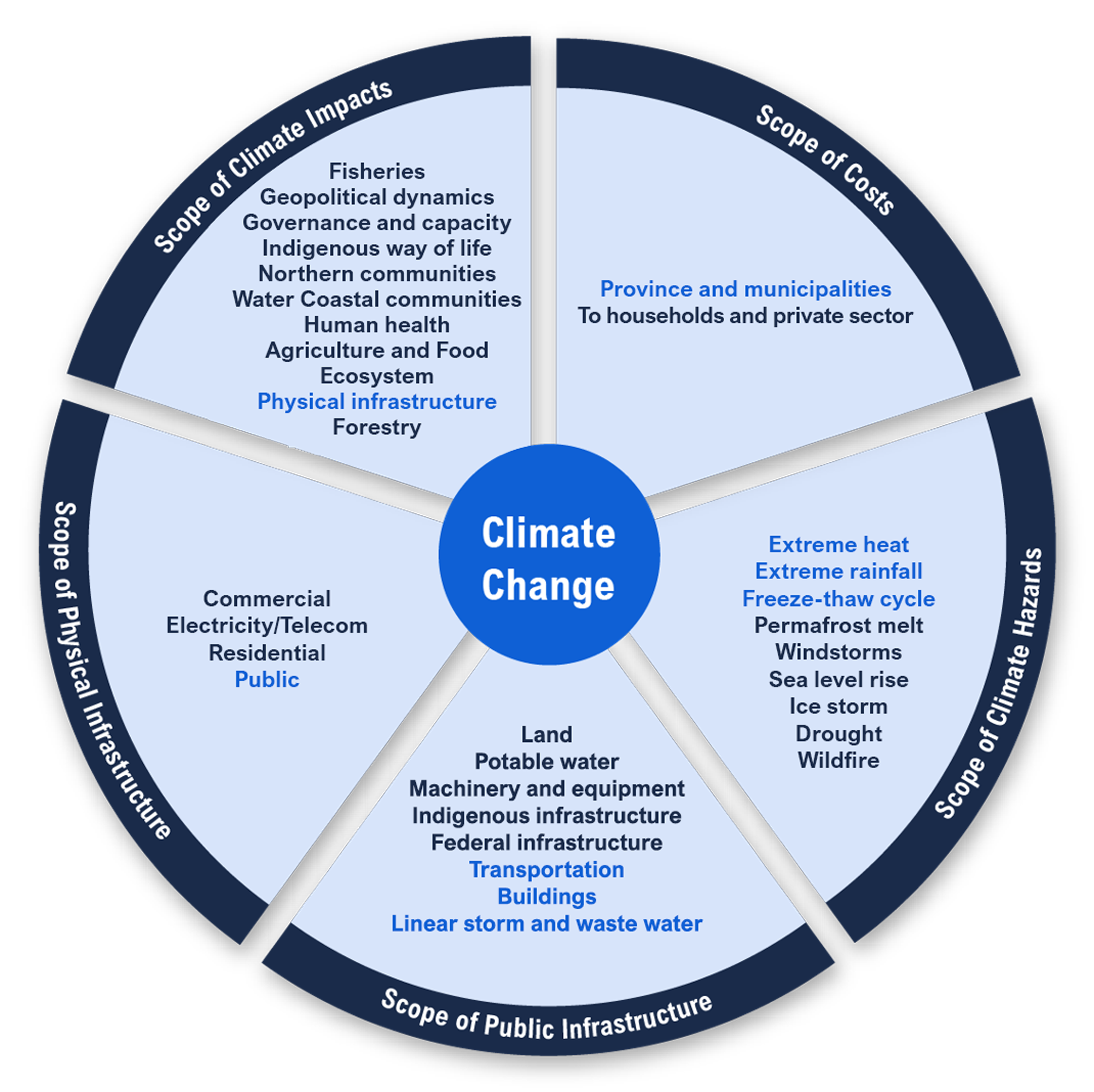
Note: Items highlighted in light blue represent the scope of costs analyzed within the CIPI project.
Source: Council of Canadian Academies and FAO.
CIPI’s results should be seen as lower-bound cost impacts
Given CIPI’s limited scope, the cost impacts of climate change on the Province and Ontario’s municipalities are likely to be larger. There are many reasons that CIPI’s climate-related infrastructure cost projections are underestimated given the broader scope of climate change’s impacts to public infrastructure.
CIPI examined a subset of public infrastructure in Ontario
The CIPI project focused on public buildings, transportation, and linear storm and wastewater infrastructure owned by provincial and municipal governments (see Figure 3‑1). While these assets make up the majority of Ontario’s public infrastructure portfolio, many public asset classes were excluded, including linear drinking water infrastructure, machinery and equipment, land, assets owned by the federal government, and assets owned by Indigenous communities. While changing climate hazards will impact these assets, they were excluded from the FAO’s analysis due to data availability, materiality and the FAO’s own resource constraints.
CIPI analyzed only three climate hazards
CIPI focused on the impacts of three climate hazards: extreme heat, extreme rainfall and freeze-thaw cycles (see Figure 3‑3). Other climate hazards, including fluvial flooding, wildfires and permafrost melt (among others), will impact public infrastructure but were excluded from the analysis either due to data availability, a lack of confidence in forecasting certain climate hazards or cost materiality.
CIPI excluded costs to households and businesses
CIPI focused on the direct costs to government budgets of maintaining infrastructure in a state of good repair. However, climate change’s impact on unadapted public infrastructure will have broader societal costs that will impact households and businesses. These costs were beyond the CIPI project’s scope but are likely to be significant. As such, these costs are an area for further research that could greatly benefit the public interest.
CIPI modelling assumptions, taken together, produced more conservative estimates
CIPI’s modelling approach allowed for significant flexibility in evaluating the impact of climate change costs to public infrastructure, including the ability to model cost outcomes in different emissions scenarios, for different cost types (i.e., O&M, rehabilitation or renewal costs), and for various geographies. CIPI’s modelling approach also had numerous limitations that, taken together, produced conservative cost estimates.
CIPI’s approach assessed the impact of each climate hazard independently and did not account for the significant interdependencies between public infrastructure. Extreme weather events often cause cascading infrastructure failures, such as storms that knock out power to sump pumps in public buildings, leading to significant damage from basement flooding. The inability to adequately model these interdependencies is one reason that CIPI’s climate costs (and those under the no adaptation strategy in particular) should be considered lower-bound estimates.
CIPI assumed that all assets are kept in a state of good repair and that whatever capital investment or operating spending is needed is available and spent by the Province and Ontario’s municipalities. However, significant infrastructure backlogs exist, and assets in poorer condition may be more vulnerable to climate hazards, leading to higher climate-related costs to maintain infrastructure and higher broader societal climate-related costs.
Lastly, CIPI used the most recent climate model projections available from Environment and Climate Change Canada at the time of the analysis. These projections, based on global climate models developed by modelling centres around the world, show a roughly linear path for global warming. They do not anticipate any potential climatic “tipping points,” or thresholds beyond which aspects of the climate system could reorganize and not return to their historical state. These tipping points could have dramatic impacts, including on the costs to maintain public infrastructure.
9 | Results Appendix
| Portfolio | Stable Climate Base Case Average Annual Costs, 2022-2100 (billions, 2020$) | Average annual climate-related infrastructure costs (2022-2100, billions, 2020$) | |||||||||
|---|---|---|---|---|---|---|---|---|---|---|---|
| Low Emissions Scenario | Medium Emissions Scenario | High Emissions Scenario | |||||||||
| Lower Bound* (0.8°C)** | Median (1.6°C) | Upper Bound (2.4°C) | Lower Bound (1.7°C) | Median (2.3°C) | Upper Bound (3.2°C) | Lower Bound (3.2°C) | Median (4.2°C) | Upper Bound (5.4°C) | |||
| Total | $26.0 | No Adaptation | $1.2 | $2.8 | $5.1 | $2.1 | $4.1 | $7.6 | $4.0 | $7.4 | $12.8 |
| Proactive Adaptation | $0.8 | $1.8 | $3.7 | $1.4 | $3.0 | $5.5 | $3.0 | $5.7 | $9.8 | ||
| Reactive Adaptation | $1.1 | $2.4 | $4.6 | $1.8 | $3.5 | $6.4 | $3.3 | $5.9 | $10.2 | ||
| Municipal | $17.8 | No Adaptation | $0.9 | $2.2 | $4.1 | $1.7 | $3.3 | $6.0 | $3.2 | $5.9 | $10.1 |
| Proactive Adaptation | $0.7 | $1.5 | $3.0 | $1.2 | $2.4 | $4.4 | $2.5 | $4.6 | $7.9 | ||
| Reactive Adaptation | $0.9 | $2.0 | $3.8 | $1.6 | $2.9 | $5.3 | $2.9 | $4.9 | $8.4 | ||
| Provincial | $8.2 | No Adaptation | $0.2 | $0.6 | $1.0 | $0.3 | $0.8 | $1.5 | $0.7 | $1.5 | $2.7 |
| Proactive Adaptation | $0.1 | $0.4 | $0.7 | $0.2 | $0.6 | $1.1 | $0.5 | $1.1 | $1.9 | ||
| Reactive Adaptation | $0.1 | $0.4 | $0.8 | $0.2 | $0.6 | $1.1 | $0.5 | $1.0 | $1.7 | ||
| Buildings | $10.1 | No Adaptation | $0.2 | $0.5 | $1.1 | $0.4 | $0.8 | $1.7 | $0.7 | $1.5 | $2.9 |
| Proactive Adaptation | $0.2 | $0.4 | $0.9 | $0.3 | $0.7 | $1.2 | $0.6 | $1.3 | $2.2 | ||
| Reactive Adaptation | $0.2 | $0.4 | $0.9 | $0.3 | $0.7 | $1.4 | $0.6 | $1.2 | $2.2 | ||
| Transportation | $12.9 | No Adaptation | $0.6 | $1.5 | $2.4 | $1.1 | $2.2 | $3.8 | $2.3 | $4.1 | $6.6 |
| Proactive Adaptation | $0.3 | $0.8 | $1.7 | $0.6 | $1.4 | $2.7 | $1.4 | $2.7 | $4.9 | ||
| Reactive Adaptation | $0.5 | $1.2 | $2.1 | $0.8 | $1.7 | $3.0 | $1.6 | $2.9 | $4.7 | ||
| Linear Storm and Wastewater | $3.0 | No Adaptation | $0.4 | $0.8 | $1.6 | $0.6 | $1.1 | $2.1 | $1.0 | $1.8 | $3.3 |
| Proactive Adaptation | $0.3 | $0.6 | $1.2 | $0.5 | $0.9 | $1.6 | $1.0 | $1.6 | $2.8 | ||
| Reactive Adaptation | $0.4 | $0.8 | $1.5 | $0.6 | $1.1 | $2.1 | $1.1 | $1.9 | $3.2 | ||
Definitions
- The no adaptation strategy assumes that public infrastructure is not adapted to withstand changing climate hazards, and instead, asset managers pay the higher costs of maintaining assets in a state of good repair in the face of increasing climate hazards.
- The proactive adaptation strategy assumes that infrastructure is adapted at the first available opportunity, and that the portfolio is fully adapted by 2070.
- The reactive adaptation strategy assumes that infrastructure assets are adapted when replaced at the end of their useful lives, and that half of the portfolio is adapted by 2070.
- The low emissions scenario assumes a major and immediate turnaround in global climate policies.
- The medium emissions scenario assumes that global emissions peak in the 2040s, then decline rapidly thereafter.
- The high emissions scenario assumes global emissions continue to grow at their historical pace for most of the century.
| Net Debt-to-GDP Impact (percentage points)*** | Asset Management Strategy |
Low Emissions Scenario | Medium Emissions Scenario | High Emissions Scenario | |||||||
|---|---|---|---|---|---|---|---|---|---|---|---|
| Lower Bound* (0.8°C)** | Median (1.6°C) | Upper Bound (2.4°C) | Lower Bound (1.7°C) | Median (2.3°C) | Upper Bound (3.2°C) | Lower Bound (3.2°C) | Median (4.2°C) | Upper Bound (5.4°C) | |||
| No Adaptation | 2020s | 0.1 | 0.2 | 0.3 | 0.1 | 0.2 | 0.4 | 0.1 | 0.2 | 0.4 | |
| 2030s | 0.3 | 0.8 | 1.4 | 0.3 | 0.8 | 1.6 | 0.4 | 1.0 | 1.7 | ||
| 2040s | 0.4 | 1.3 | 2.2 | 0.6 | 1.4 | 2.7 | 0.6 | 1.7 | 3.0 | ||
| 2050s | 0.6 | 1.6 | 2.8 | 0.8 | 1.9 | 3.5 | 1.1 | 2.4 | 4.0 | ||
| 2060s | 0.7 | 1.8 | 3.3 | 1.0 | 2.3 | 4.4 | 1.4 | 3.1 | 5.4 | ||
| 2070s | 0.7 | 2.1 | 3.9 | 1.1 | 2.8 | 5.2 | 1.8 | 3.9 | 6.7 | ||
| 2080s | 0.8 | 2.3 | 4.3 | 1.3 | 3.1 | 5.9 | 2.2 | 4.6 | 8.0 | ||
| 2090s | 0.9 | 2.5 | 4.6 | 1.4 | 3.4 | 6.4 | 2.6 | 5.4 | 9.4 | ||
| Proactive Adaptation | 2020s | 0.1 | 0.3 | 0.6 | 0.2 | 0.4 | 0.8 | 0.4 | 0.7 | 1.2 | |
| 2030s | 0.5 | 1.1 | 2.2 | 0.7 | 1.6 | 3.1 | 1.4 | 2.8 | 4.8 | ||
| 2040s | 0.6 | 1.5 | 2.9 | 1.0 | 2.3 | 4.1 | 2.1 | 4.1 | 6.9 | ||
| 2050s | 0.8 | 1.8 | 3.4 | 1.3 | 2.8 | 4.9 | 2.7 | 4.9 | 8.2 | ||
| 2060s | 0.8 | 1.8 | 3.5 | 1.3 | 2.8 | 5.1 | 2.8 | 5.2 | 8.7 | ||
| 2070s | 0.7 | 1.7 | 3.6 | 1.2 | 2.8 | 5.2 | 2.8 | 5.3 | 9.0 | ||
| 2080s | 0.8 | 1.9 | 3.8 | 1.3 | 3.0 | 5.5 | 2.8 | 5.5 | 9.4 | ||
| 2090s | 0.7 | 1.9 | 3.8 | 1.2 | 3.0 | 5.5 | 2.8 | 5.5 | 9.5 | ||
| Reactive Adaptation | 2020s | 0.1 | 0.2 | 0.3 | 0.1 | 0.2 | 0.4 | 0.1 | 0.2 | 0.4 | |
| 2030s | 0.3 | 0.8 | 1.5 | 0.3 | 0.9 | 1.7 | 0.4 | 1.1 | 1.9 | ||
| 2040s | 0.4 | 1.3 | 2.4 | 0.6 | 1.6 | 2.9 | 0.9 | 2.1 | 3.6 | ||
| 2050s | 0.6 | 1.6 | 2.9 | 0.9 | 2.0 | 3.7 | 1.4 | 2.8 | 4.7 | ||
| 2060s | 0.7 | 1.7 | 3.2 | 1.0 | 2.3 | 4.3 | 1.6 | 3.4 | 5.9 | ||
| 2070s | 0.6 | 1.9 | 3.6 | 1.0 | 2.5 | 4.8 | 1.9 | 3.9 | 6.6 | ||
| 2080s | 0.7 | 2.0 | 3.8 | 1.1 | 2.7 | 5.1 | 2.0 | 4.2 | 7.3 | ||
| 2090s | 0.7 | 2.0 | 3.9 | 1.1 | 2.8 | 5.2 | 2.0 | 4.3 | 7.5 | ||
Definitions
- The no adaptation strategy assumes that public infrastructure is not adapted to withstand changing climate hazards, and instead, asset managers pay the higher costs of maintaining assets in a state of good repair in the face of increasing climate hazards.
- The proactive adaptation strategy assumes that infrastructure is adapted at the first available opportunity, and that the portfolio is fully adapted by 2070.
- The reactive adaptation strategy assumes that infrastructure assets are adapted when replaced at the end of their useful lives, and that half of the portfolio is adapted by 2070.
- The low emissions scenario assumes a major and immediate turnaround in global climate policies.
- The medium emissions scenario assumes that global emissions peak in the 2040s, then decline rapidly thereafter.
- The high emissions scenario assumes global emissions continue to grow at their historical pace for most of the century.
| Interest on Debt-to-Revenue Impact (percentage points)*** | Asset Management Strategy |
Low Emissions Scenario | Medium Emissions Scenario | High Emissions Scenario | |||||||
|---|---|---|---|---|---|---|---|---|---|---|---|
| Lower Bound* (0.8°C)** | Median (1.6°C) | Upper Bound (2.4°C) | Lower Bound (1.7°C) | Median (2.3°C) | Upper Bound (3.2°C) | Lower Bound (3.2°C) | Median (4.2°C) | Upper Bound (5.4°C) | |||
| No Adaptation | 2020s | 0.0 | 0.0 | 0.1 | 0.0 | 0.0 | 0.1 | 0.0 | 0.0 | 0.1 | |
| 2030s | 0.1 | 0.2 | 0.3 | 0.1 | 0.2 | 0.3 | 0.1 | 0.2 | 0.3 | ||
| 2040s | 0.1 | 0.3 | 0.4 | 0.1 | 0.3 | 0.5 | 0.1 | 0.3 | 0.6 | ||
| 2050s | 0.1 | 0.3 | 0.6 | 0.2 | 0.4 | 0.7 | 0.2 | 0.5 | 0.8 | ||
| 2060s | 0.1 | 0.4 | 0.7 | 0.2 | 0.5 | 0.9 | 0.3 | 0.6 | 1.1 | ||
| 2070s | 0.1 | 0.4 | 0.8 | 0.2 | 0.6 | 1.1 | 0.4 | 0.8 | 1.3 | ||
| 2080s | 0.2 | 0.5 | 0.9 | 0.3 | 0.6 | 1.2 | 0.4 | 0.9 | 1.6 | ||
| 2090s | 0.2 | 0.5 | 0.9 | 0.3 | 0.7 | 1.3 | 0.5 | 1.1 | 1.9 | ||
| Proactive Adaptation | 2020s | 0.0 | 0.1 | 0.1 | 0.0 | 0.1 | 0.2 | 0.1 | 0.1 | 0.2 | |
| 2030s | 0.1 | 0.2 | 0.4 | 0.1 | 0.3 | 0.6 | 0.3 | 0.6 | 1.0 | ||
| 2040s | 0.1 | 0.3 | 0.6 | 0.2 | 0.5 | 0.8 | 0.4 | 0.8 | 1.4 | ||
| 2050s | 0.2 | 0.4 | 0.7 | 0.3 | 0.6 | 1.0 | 0.5 | 1.0 | 1.7 | ||
| 2060s | 0.2 | 0.4 | 0.7 | 0.3 | 0.6 | 1.0 | 0.6 | 1.0 | 1.7 | ||
| 2070s | 0.1 | 0.4 | 0.7 | 0.2 | 0.6 | 1.1 | 0.6 | 1.1 | 1.8 | ||
| 2080s | 0.2 | 0.4 | 0.8 | 0.3 | 0.6 | 1.1 | 0.6 | 1.1 | 1.9 | ||
| 2090s | 0.1 | 0.4 | 0.8 | 0.2 | 0.6 | 1.1 | 0.6 | 1.1 | 1.9 | ||
| Reactive Adaptation | 2020s | 0.0 | 0.0 | 0.1 | 0.0 | 0.0 | 0.1 | 0.0 | 0.0 | 0.1 | |
| 2030s | 0.1 | 0.2 | 0.3 | 0.1 | 0.2 | 0.3 | 0.1 | 0.2 | 0.4 | ||
| 2040s | 0.1 | 0.3 | 0.5 | 0.1 | 0.3 | 0.6 | 0.2 | 0.4 | 0.7 | ||
| 2050s | 0.1 | 0.3 | 0.6 | 0.2 | 0.4 | 0.7 | 0.3 | 0.6 | 0.9 | ||
| 2060s | 0.1 | 0.3 | 0.6 | 0.2 | 0.5 | 0.9 | 0.3 | 0.7 | 1.2 | ||
| 2070s | 0.1 | 0.4 | 0.7 | 0.2 | 0.5 | 1.0 | 0.4 | 0.8 | 1.3 | ||
| 2080s | 0.1 | 0.4 | 0.8 | 0.2 | 0.5 | 1.0 | 0.4 | 0.8 | 1.5 | ||
| 2090s | 0.1 | 0.4 | 0.8 | 0.2 | 0.6 | 1.0 | 0.4 | 0.9 | 1.5 | ||
Definitions
- The no adaptation strategy assumes that public infrastructure is not adapted to withstand changing climate hazards, and instead, asset managers pay the higher costs of maintaining assets in a state of good repair in the face of increasing climate hazards.
- The proactive adaptation strategy assumes that infrastructure is adapted at the first available opportunity, and that the portfolio is fully adapted by 2070.
- The reactive adaptation strategy assumes that infrastructure assets are adapted when replaced at the end of their useful lives, and that half of the portfolio is adapted by 2070.
- The low emissions scenario assumes a major and immediate turnaround in global climate policies.
- The medium emissions scenario assumes that global emissions peak in the 2040s, then decline rapidly thereafter.
- The high emissions scenario assumes global emissions continue to grow at their historical pace for most of the century.
| Net Debt-to-GDP Impact (percentage points)*** | Asset Management Strategy |
Emissions Scenario | Low Emissions Scenario | Medium Emissions Scenario | High Emissions Scenario | ||||||
|---|---|---|---|---|---|---|---|---|---|---|---|
| Lower Bound* (0.8°C)** | Median (1.6°C) | Upper Bound (2.4°C) | Lower Bound (1.7°C) | Median (2.3°C) | Upper Bound (3.2°C) | Lower Bound (3.2°C) | Median (4.2°C) | Upper Bound (5.4°C) | |||
| No Adaptation | 2020s | 0.4 | 0.7 | 1.2 | 0.4 | 0.8 | 1.4 | 0.5 | 1.0 | 1.4 | |
| 2030s | 1.6 | 3.4 | 5.8 | 2.0 | 3.8 | 6.7 | 2.3 | 4.5 | 7.1 | ||
| 2040s | 2.3 | 5.5 | 9.3 | 3.2 | 6.3 | 11.5 | 3.9 | 7.8 | 12.7 | ||
| 2050s | 2.9 | 7.2 | 12.7 | 4.2 | 9.0 | 16.1 | 6.1 | 11.7 | 18.7 | ||
| 2060s | 3.9 | 9.5 | 16.9 | 6.1 | 12.4 | 21.6 | 9.4 | 16.0 | 26.7 | ||
| 2070s | 4.3 | 10.4 | 18.2 | 6.7 | 13.8 | 24.6 | 10.9 | 19.4 | 31.6 | ||
| 2080s | 4.6 | 10.8 | 19.8 | 7.0 | 14.8 | 27.3 | 12.2 | 22.6 | 37.8 | ||
| 2090s | 4.9 | 11.9 | 21.6 | 8.0 | 16.7 | 29.9 | 14.4 | 26.3 | 44.5 | ||
| Proactive Adaptation | 2020s | 1.3 | 1.9 | 3.1 | 1.7 | 2.6 | 4.1 | 2.7 | 4.1 | 6.3 | |
| 2030s | 4.4 | 6.8 | 11.2 | 5.7 | 9.1 | 14.9 | 9.2 | 14.6 | 23.1 | ||
| 2040s | 7.4 | 10.6 | 16.6 | 9.4 | 14.1 | 21.9 | 14.6 | 22.1 | 34.2 | ||
| 2050s | 9.0 | 12.9 | 19.8 | 11.4 | 17.0 | 26.1 | 17.6 | 26.6 | 40.9 | ||
| 2060s | 8.4 | 12.8 | 20.4 | 11.0 | 17.3 | 27.4 | 17.9 | 27.8 | 43.8 | ||
| 2070s | 7.8 | 12.2 | 20.5 | 10.6 | 17.1 | 28.0 | 18.0 | 28.7 | 46.0 | ||
| 2080s | 6.8 | 11.4 | 19.9 | 9.5 | 16.5 | 27.7 | 17.1 | 28.4 | 46.4 | ||
| 2090s | 6.2 | 11.0 | 19.8 | 8.9 | 16.2 | 27.9 | 16.7 | 28.5 | 47.2 | ||
| Reactive Adaptation | 2020s | 0.4 | 0.7 | 1.3 | 0.5 | 0.9 | 1.5 | 0.6 | 1.1 | 1.8 | |
| 2030s | 1.6 | 3.4 | 5.8 | 2.0 | 3.9 | 6.8 | 2.5 | 4.8 | 7.6 | ||
| 2040s | 2.2 | 5.3 | 9.2 | 3.2 | 6.3 | 11.5 | 4.2 | 8.3 | 13.5 | ||
| 2050s | 2.8 | 7.0 | 12.5 | 4.2 | 8.9 | 16.1 | 6.5 | 12.4 | 20.1 | ||
| 2060s | 3.9 | 9.3 | 16.9 | 6.1 | 12.5 | 21.9 | 10.2 | 17.3 | 29.6 | ||
| 2070s | 4.3 | 10.1 | 17.9 | 6.7 | 13.8 | 24.7 | 11.6 | 20.7 | 33.9 | ||
| 2080s | 4.4 | 10.1 | 18.9 | 6.8 | 14.1 | 26.0 | 12.0 | 22.1 | 37.0 | ||
| 2090s | 4.6 | 10.9 | 20.0 | 7.3 | 15.2 | 27.5 | 13.2 | 23.9 | 40.3 | ||
Definitions
- The no adaptation strategy assumes that public infrastructure is not adapted to withstand changing climate hazards, and instead, asset managers pay the higher costs of maintaining assets in a state of good repair in the face of increasing climate hazards.
- The proactive adaptation strategy assumes that infrastructure is adapted at the first available opportunity, and that the portfolio is fully adapted by 2070.
- The reactive adaptation strategy assumes that infrastructure assets are adapted when replaced at the end of their useful lives, and that half of the portfolio is adapted by 2070.
- The low emissions scenario assumes a major and immediate turnaround in global climate policies.
- The medium emissions scenario assumes that global emissions peak in the 2040s, then decline rapidly thereafter.
- The high emissions scenario assumes global emissions continue to grow at their historical pace for most of the century.
| Interest on Debt-to-Revenue Impact (percentage points)*** | Asset Management Strategy |
Emissions Scenario | Low Emissions Scenario | Medium Emissions Scenario | High Emissions Scenario | ||||||
|---|---|---|---|---|---|---|---|---|---|---|---|
| Lower Bound* (0.8°C)** | Median (1.6°C) | Upper Bound (2.4°C) | Lower Bound (1.7°C) | Median (2.3°C) | Upper Bound (3.2°C) | Lower Bound (3.2°C) | Median (4.2°C) | Upper Bound (5.4°C) | |||
| No Adaptation | 2020s | 0.1 | 0.1 | 0.2 | 0.1 | 0.2 | 0.3 | 0.1 | 0.2 | 0.3 | |
| 2030s | 0.3 | 0.7 | 1.2 | 0.4 | 0.8 | 1.4 | 0.5 | 0.9 | 1.4 | ||
| 2040s | 0.5 | 1.1 | 1.9 | 0.6 | 1.3 | 2.3 | 0.8 | 1.6 | 2.6 | ||
| 2050s | 0.6 | 1.5 | 2.6 | 0.9 | 1.8 | 3.3 | 1.2 | 2.4 | 3.8 | ||
| 2060s | 0.8 | 1.9 | 3.4 | 1.2 | 2.5 | 4.4 | 1.9 | 3.2 | 5.4 | ||
| 2070s | 0.9 | 2.1 | 3.7 | 1.4 | 2.8 | 5.0 | 2.2 | 3.9 | 6.4 | ||
| 2080s | 0.9 | 2.2 | 4.0 | 1.4 | 3.0 | 5.5 | 2.5 | 4.6 | 7.7 | ||
| 2090s | 1.0 | 2.4 | 4.4 | 1.6 | 3.4 | 6.0 | 2.9 | 5.3 | 9.0 | ||
| Proactive Adaptation | 2020s | 0.3 | 0.4 | 0.6 | 0.3 | 0.5 | 0.8 | 0.5 | 0.8 | 1.3 | |
| 2030s | 0.9 | 1.4 | 2.3 | 1.1 | 1.9 | 3.0 | 1.9 | 3.0 | 4.7 | ||
| 2040s | 1.5 | 2.1 | 3.4 | 1.9 | 2.8 | 4.4 | 2.9 | 4.5 | 6.9 | ||
| 2050s | 1.8 | 2.6 | 4.0 | 2.3 | 3.4 | 5.3 | 3.6 | 5.4 | 8.3 | ||
| 2060s | 1.7 | 2.6 | 4.1 | 2.2 | 3.5 | 5.6 | 3.6 | 5.6 | 8.9 | ||
| 2070s | 1.6 | 2.5 | 4.1 | 2.1 | 3.5 | 5.7 | 3.6 | 5.8 | 9.3 | ||
| 2080s | 1.4 | 2.3 | 4.0 | 1.9 | 3.3 | 5.6 | 3.5 | 5.7 | 9.4 | ||
| 2090s | 1.3 | 2.2 | 4.0 | 1.8 | 3.3 | 5.7 | 3.4 | 5.8 | 9.6 | ||
| Reactive Adaptation | 2020s | 0.1 | 0.1 | 0.3 | 0.1 | 0.2 | 0.3 | 0.1 | 0.2 | 0.4 | |
| 2030s | 0.3 | 0.7 | 1.2 | 0.4 | 0.8 | 1.4 | 0.5 | 1.0 | 1.5 | ||
| 2040s | 0.4 | 1.1 | 1.9 | 0.6 | 1.3 | 2.3 | 0.8 | 1.7 | 2.7 | ||
| 2050s | 0.6 | 1.4 | 2.5 | 0.8 | 1.8 | 3.3 | 1.3 | 2.5 | 4.1 | ||
| 2060s | 0.8 | 1.9 | 3.4 | 1.2 | 2.5 | 4.4 | 2.1 | 3.5 | 6.0 | ||
| 2070s | 0.9 | 2.0 | 3.6 | 1.4 | 2.8 | 5.0 | 2.3 | 4.2 | 6.9 | ||
| 2080s | 0.9 | 2.0 | 3.8 | 1.4 | 2.8 | 5.2 | 2.4 | 4.5 | 7.5 | ||
| 2090s | 0.9 | 2.2 | 4.0 | 1.5 | 3.1 | 5.5 | 2.7 | 4.8 | 8.1 | ||
Definitions
- The no adaptation strategy assumes that public infrastructure is not adapted to withstand changing climate hazards, and instead, asset managers pay the higher costs of maintaining assets in a state of good repair in the face of increasing climate hazards.
- The proactive adaptation strategy assumes that infrastructure is adapted at the first available opportunity, and that the portfolio is fully adapted by 2070.
- The reactive adaptation strategy assumes that infrastructure assets are adapted when replaced at the end of their useful lives, and that half of the portfolio is adapted by 2070.
- The low emissions scenario assumes a major and immediate turnaround in global climate policies.
- The medium emissions scenario assumes that global emissions peak in the 2040s, then decline rapidly thereafter.
- The high emissions scenario assumes global emissions continue to grow at their historical pace for most of the century.
10 | References
Canadian Standards Association (2014). Canadian Highway Bridge Design Code.
Climate Risk Institute and Dillon Consulting Limited (2023). Ontario Provincial Climate Change Impact Assessment Technical Report.
Council of Canadian Academies (2019). Canada’s Top Climate Change Risks.
Financial Accountability Office of Ontario (2020). Provincial Infrastructure.
Financial Accountability Office of Ontario (2021). Municipal Infrastructure.
Financial Accountability Office of Ontario (2021). Costing Climate Change Impacts to Public Infrastructure: Assessing the financial impacts of extreme rainfall, extreme heat and freeze-thaw cycles on public buildings in Ontario.
Financial Accountability Office of Ontario (2021). Costing Climate Change Impacts to Public Infrastructure: Project Backgrounder and Methodology.
Financial Accountability Office of Ontario (2021).Costing Climate Change Impacts to Public Infrastructure: WSP Engineering Report.
Financial Accountability Office of Ontario (2022). Costing Climate Change Impacts to Public Infrastructure: Assessing the financial impacts of extreme rainfall, extreme heat and freeze-thaw cycles on transportation infrastructure in Ontario.
Financial Accountability Office of Ontario (2022). Costing Climate Change Impacts to Public Infrastructure: Assessing the financial impacts of extreme rainfall on public linear storm and wastewater infrastructure in Ontario.
Financial Accountability Office of Ontario (2022). Long-Term Budget Outlook: Assessing Ontario’s Fiscal Sustainability: 2021-2050.
Government of Canada: Environment and Climate Change Canada (2023). National Adaptation Strategy.
Government of Canada: Environment and Climate Change Canada (2023). Climate Data for a Resilient Canada.
Government of Canada: Infrastructure Canada (2019). Climate Change Resilience Assessment.
Intergovernmental Panel on Climate Change (2013).Climate Change 2013: The Physical Science Basis.
Intergovernmental Panel on Climate Change (2015). Climate Change 2014: Synthesis Report.
Office of the Auditor General of Ontario (2022).Value-for-Money Audit: Climate Change Adaptation: Reducing Urban Flood Risk.
Prairie Climate Centre (2023). Climate Atlas of Canada.
Statistics Canada (2016). Standard Geographical Classification (SGC) 2016 – Introduction: Economic Regions – Variant of SGC 2016.
United Nations Environment Programme (2022).Emissions Gap Report.
Warren, F.J. and Lulham, N., editors (2021). Canada in a Changing Climate: National Issues Report, Government of Canada.
Graphical Descriptions
| Stable Climate Base Case | Medium Emissions Scenario, No Adaptation | ||||
|---|---|---|---|---|---|
| Average annual infrastructure spending (2022-2100, Billions 2020$) | Per cent change | ||||
| Total | $26.0 | +$4.1 | 16% | ||
| Level of government | Municipal | $17.8 | +$3.3 | 18% | |
| Provincial | $8.2 | +$0.8 | 10% | ||
| Asset type | Buildings | $10.1 | +$0.8 | 8% | |
| Transportation | $12.9 | +$2.2 | 17% | ||
| Linear Storm and Wastewater | $3.0 | +$1.1 | 37% | ||
| Average annual climate-related infrastructure costs (2022-2100) | Difference in average annual climate-related infrastructure costs (2022-2100) from No Adaptation Strategy | ||
|---|---|---|---|
| Infrastructure costs (2020$ billions) | Per cent increase from stable climate base case | Infrastructure costs (2020$ billions) | |
| No Adaptation | $4.1 | 16% | - |
| Reactive Adaptation | $3.5 | 13% | -$0.6 |
| Proactive Adaptation | $3.0 | 11% | -$1.1 |
| Share of total adapted infrastructure by current replacement value (Per Cent) | |||
|---|---|---|---|
| Year | No Adaptation | Reactive Adaptation | Proactive Adaptation |
| 2022 | 0 | 6 | 12 |
| 2030 | 0 | 7 | 43 |
| 2040 | 0 | 12 | 79 |
| 2050 | 0 | 19 | 92 |
| 2060 | 0 | 28 | 99 |
| 2070 | 0 | 54 | 100 |
| 2080 | 0 | 71 | 100 |
| 2090 | 0 | 81 | 100 |
| 2100 | 0 | 87 | 100 |
| Change in Ontario's net debt-to-GDP ratio (Percentage points) under the medium emissions scenario | |||
|---|---|---|---|
| Decade | No Adaptation | Reactive Adaptation | Proactive Adaptation |
| 2020s | 0.2% | 0.2% | 0.4% |
| 2030s | 0.8% | 0.9% | 1.6% |
| 2040s | 1.4% | 1.6% | 2.3% |
| 2050s | 1.9% | 2.0% | 2.8% |
| 2060s | 2.3% | 2.3% | 2.8% |
| 2070s | 2.8% | 2.5% | 2.8% |
| 2080s | 3.1% | 2.7% | 3.0% |
| 2090s | 3.4% | 2.8% | 3.0% |
| Change in Ontario's net debt-to-GDP ratio (percentage points) under the medium emissions scenario | |||
|---|---|---|---|
| Decade | No Adaptation | Reactive Adaptation | Proactive Adaptation |
| 2020s | 0.8% | 0.9% | 2.6% |
| 2030s | 3.8% | 3.9% | 9.1% |
| 2040s | 6.3% | 6.3% | 14.1% |
| 2050s | 9.0% | 8.9% | 17.0% |
| 2060s | 12.4% | 12.5% | 17.3% |
| 2070s | 13.8% | 13.8% | 17.1% |
| 2080s | 14.8% | 14.1% | 16.5% |
| 2090s | 16.7% | 15.2% | 16.2% |
| Year | CIPI Project Report |
|---|---|
| 2020 | Provincial Infrastructure |
| 2021 | Municipal Infrastructure |
| Project Backgrounder and Methodology | |
| WSP Report | |
| Buildings and Facilities | |
| 2022 | Public Transportation Infrastructure |
| Public Linear Storm and Wastewater Infrastructure | |
| 2023 | Summary Report |
| Level of government | Infrastructure type | Value (in billions of $) | Per cent of total |
|---|---|---|---|
| Municipal | Transportation | $269 | 38% |
| Linear Storm and Wastewater | $124 | 17% | |
| Buildings | $113 | 16% | |
| Provincial | Transportation | $61 | 9% |
| Buildings | $141 | 20% |
| Time Period | Change in Global Mean Temperature Relative to Pre-Industrial Level Relative to Pre-Industrial Level (°C) | ||||||||||
|---|---|---|---|---|---|---|---|---|---|---|---|
| Historical | Stable Climate Base Case | Low Emissions Scenario | Medium Emissions Scenario | High Emissions Scenario | |||||||
| Low | Median | High | Low | Median | High | Low | Median | High | |||
| Pre-industrial period* | 0 | ||||||||||
| 1976-2005 | 0.5 | 0.5 | |||||||||
| 2010 | 1.0 | 0.5 | |||||||||
| 2020 | 1.2 | 0.5 | |||||||||
| 2030 | 0.5 | 1.1 | 1.4 | 1.9 | 1.2 | 1.4 | 1.8 | 1.3 | 1.6 | 2.0 | |
| 2040 | 0.5 | 1.1 | 1.5 | 2.1 | 1.3 | 1.7 | 2.2 | 1.5 | 1.9 | 2.4 | |
| 2050 | 0.5 | 1.1 | 1.6 | 2.3 | 1.5 | 1.9 | 2.6 | 1.8 | 2.3 | 3.0 | |
| 2060 | 0.5 | 1.0 | 1.5 | 2.3 | 1.5 | 2.1 | 2.8 | 2.2 | 2.8 | 3.6 | |
| 2070 | 0.5 | 0.8 | 1.5 | 2.3 | 1.6 | 2.2 | 2.9 | 2.6 | 3.2 | 4.2 | |
| 2080 | 0.5 | 0.8 | 1.6 | 2.4 | 1.6 | 2.2 | 3.2 | 2.9 | 3.7 | 4.8 | |
| 2090 | 0.5 | 0.8 | 1.6 | 2.4 | 1.7 | 2.3 | 3.2 | 3.2 | 4.2 | 5.4 | |
| Asset Type | Climate Hazard | ||
|---|---|---|---|
| Extreme heat | Extreme rainfall | Freeze-thaw cycles | |
| Buildings | Included | Included | Included |
| Roads | Included | Included | Not included |
| Rail | Included | Not included | Not included |
| Bridges | Not included | Included | Included |
| Culverts | Not included | Included | Not included |
| Linear stormwater | Not included | Included | Not included |
| Linear wastewater | Not included | Included | Not included |
| Linear drinking water | Not included | Not included | Not included |
| Machinery and equipment | Not included | Not included | Not included |
| Year | Ontario annual number of days with temperature over 30°C | ||||||||
|---|---|---|---|---|---|---|---|---|---|
| Low emissions scenario | Medium emissions scenario | High emissions scenario | |||||||
| Low | Median | High | Low | Median | High | Low | Median | High | |
| 1950 | 1 | 3 | 5 | 1 | 3 | 5 | 1 | 3 | 5 |
| 1960 | 1 | 3 | 7 | 1 | 3 | 6 | 1 | 3 | 7 |
| 1970 | 1 | 3 | 7 | 1 | 2 | 6 | 1 | 3 | 7 |
| 1980 | 1 | 2 | 8 | 1 | 2 | 7 | 1 | 2 | 8 |
| 1990 | 1 | 3 | 8 | 1 | 3 | 8 | 1 | 3 | 8 |
| 2000 | 2 | 5 | 8 | 2 | 4 | 8 | 2 | 5 | 8 |
| 2010 | 2 | 4 | 10 | 3 | 5 | 9 | 3 | 5 | 9 |
| 2020 | 2 | 6 | 10 | 3 | 6 | 11 | 2 | 7 | 12 |
| 2030 | 4 | 8 | 12 | 2 | 9 | 18 | 6 | 10 | 14 |
| 2040 | 3 | 8 | 14 | 4 | 7 | 19 | 4 | 11 | 19 |
| 2050 | 4 | 9 | 20 | 4 | 12 | 21 | 8 | 15 | 30 |
| 2060 | 3 | 11 | 20 | 7 | 15 | 21 | 7 | 18 | 36 |
| 2070 | 3 | 9 | 16 | 8 | 16 | 25 | 12 | 23 | 35 |
| 2080 | 4 | 8 | 19 | 6 | 18 | 27 | 12 | 37 | 47 |
| 2090 | 4 | 9 | 19 | 8 | 16 | 33 | 20 | 41 | 61 |
| 2100 | 4 | 7 | 13 | 5 | 16 | 29 | 24 | 46 | 71 |
| Region | Projected change in annual mean temperatures from 1976-2005 to 2071-2100, median projection, medium emissions scenario |
|---|---|
| Hamilton-Niagara Peninsula | 3.1 |
| Kingston-Pembroke | 3.0 |
| Kitchener-Waterloo-Barrie | 3.1 |
| London | 3.1 |
| Muskoka-Kawarthas | 3.0 |
| Northeast A | 3.0 |
| Northeast B | 3.1 |
| Northeast C | 3.3 |
| Northwest A | 3.2 |
| Northwest B | 3.2 |
| Northwest C | 3.5 |
| Ontario | 3.3 |
| Ottawa | 3.0 |
| Stratford-Bruce Peninsula | 3.1 |
| Toronto | 3.1 |
| Windsor-Sarnia | 3.1 |
| Stable climate average annual infrastructure costs (Billions, 2020$) | ||
|---|---|---|
| Total | 26.0 | |
| Level of government | Municipal | 17.8 |
| Provincial | 8.2 | |
| Asset sector | Buildings | 10.1 |
| Transportation | 12.9 | |
| Linear Storm and Wastewater | 3.0 | |
| Years | Average annual infrastructure spending (Billions, 2020$) | Percentage change from stable climate base case | |
|---|---|---|---|
| Stable Climate Base Case | Medium Emissions Scenario, No Adaptation | ||
| 2022-2030 | $21.0 | $2.6 | +12% |
| 2031-2070 | $26.2 | $4.3 | +17% |
| 2071-2100 | $27.3 | $4.3 | +16% |
| 2022-2100 | $26.0 | $4.1 | +16% |
| Emissions level | Change in Global Mean Temperature by 2100 Relative to 1850-1900 Average (°C) | ||
|---|---|---|---|
| The range of temperature increase in the medium emissions scenario | 66 per cent chance warming will be in this range under currently enacted policies of global governments based on UN assessment | 66 per cent chance warming will be in this range if international "net-zero" ambitions are realized based on UN assessment | |
| High | 3.2 | 3.3 | 1.9 |
| Median | 2.3 | 2.8 | 1.8 |
| Low | 1.7 | 1.9 | 1.7 |
| Average annual infrastructure spending (Billions, 2020$) | Percentage change from stable climate base case | |||
|---|---|---|---|---|
| Stable Climate Base Case | Medium Emissions Scenario, No Adaptation | |||
| Total | $26.0 | +$4.1 | 16% | |
| Level of government | Municipal | $17.8 | +$3.3 | 18% |
| Provincial | $8.2 | +$0.8 | 10% | |
| Asset type | Buildings | $10.1 | +$0.8 | 8% |
| Transportation | $12.9 | +$2.2 | 17% | |
| Linear Storm and Wastewater | $3.0 | +$1.1 | 37% | |
| Average annual climate-related infrastructure costs in the no adaptation strategy (2022-2100, Billions 2020$) | |||
|---|---|---|---|
| Low Emissions Scenario | Medium Emissions Scenario | High Emissions Scenario | |
| Minimum | $1.2 | $2.1 | $4.0 |
| Median | $2.8 | $4.1 | $7.4 |
| Maximum | $5.1 | $7.6 | $12.8 |
| Years | Average Annual Climate-related Infrastructure costs in the no adaptation strategy (Billions, 2020$) | ||
|---|---|---|---|
| Low Emissions Scenario | Medium Emissions Scenario | High Emissions Scenario | |
| 2022-2030 | $2.3 | $2.6 | $3.0 |
| 2031-2070 | $3.2 | $4.3 | $5.8 |
| 2071-2100 | $2.4 | $4.3 | $10.8 |
| 2022-2100 | $2.8 | $4.1 | $7.4 |
| Years | Average annual infrastructure spending (Billions, 2020$) | Percentage change from stable climate base case | |
|---|---|---|---|
| Stable Climate Base Case | Medium Emissions Scenario, Proactive Adaptation | ||
| 2022-2030 | $21.0 | +$7.9 | +38% |
| 2031-2070 | $26.2 | +$4.2 | +16% |
| 2071-2100 | $27.3 | -$0.2 | -1% |
| 2022-2100 | $26.0 | +$3.0 | +11% |
| Years | Average annual infrastructure spending (Billions, 2020$) | Percentage change from stable climate base case | |
|---|---|---|---|
| Stable Climate Base Case | Medium Emissions Scenario, Reactive Adaptation | ||
| 2022-2030 | $21.0 | +$3.1 | +15% |
| 2031-2070 | $26.2 | +$4.4 | +17% |
| 2071-2100 | $27.3 | +$2.4 | +9% |
| 2022-2100 | $26.0 | +$3.5 | +13% |
| Year | Share of total adapted infrastructure by current replacement value (Per Cent) | ||
|---|---|---|---|
| No Adaptation | Reactive Adaptation | Proactive Adaptation | |
| 2022 | 0 | 6 | 12 |
| 2030 | 0 | 7 | 43 |
| 2040 | 0 | 12 | 79 |
| 2050 | 0 | 19 | 92 |
| 2060 | 0 | 28 | 99 |
| 2070 | 0 | 54 | 100 |
| 2080 | 0 | 71 | 100 |
| 2090 | 0 | 81 | 100 |
| 2100 | 0 | 87 | 100 |
| Average annual climate-related infrastructure costs (2022-2100) | Difference in average annual climate-related infrastructure costs (2022-2100) from No Adaptation Strategy | ||
|---|---|---|---|
| Infrastructure costs (2020$ billions) | Per cent increase from stable climate base case | Infrastructure costs (2020$ billions) | |
| No Adaptation | $4.1 | 16% | - |
| Reactive Adaptation | $3.5 | 13% | -$0.6 |
| Proactive Adaptation | $3.0 | 11% | -$1.1 |
| Increase in Global Mean Surface Temperature by 2100 from 1850-1900 average (Degrees Celsius) | Average annual cost reductions compared to the no adaptation strategy (2022-2100, billions 2020$) | |
|---|---|---|
| Proactive Adaptation | Reactive Adaptation | |
| 0.8 | 0.5 | 0.2 |
| 0.3 | 0.1 | |
| 0.6 | 0.2 | |
| 1.6 | 1.0 | 0.4 |
| 0.7 | 0.2 | |
| 1.2 | 0.4 | |
| 1.7 | 0.8 | 0.4 |
| 0.7 | 0.3 | |
| 1.0 | 0.4 | |
| 2.3 | 1.1 | 0.6 |
| 0.9 | 0.5 | |
| 1.5 | 0.7 | |
| 2.4 | 1.3 | 0.5 |
| 1.0 | 0.4 | |
| 1.4 | 0.5 | |
| 3.2 | 1.7 | 0.9 |
| 1.3 | 0.6 | |
| 2.1 | 1.2 | |
| 3.2 | 1.3 | 1.0 |
| 0.9 | 0.7 | |
| 1.6 | 1.2 | |
| 4.2 | 1.7 | 1.5 |
| 1.1 | 1.0 | |
| 2.2 | 1.9 | |
| 5.4 | 2.4 | 2.0 |
| 1.5 | 1.4 | |
| 3.0 | 2.6 | |
| Decade | Change in Net Debt-to-GDP ratio (Percentage points) under the medium emissions scenario | ||
|---|---|---|---|
| No Adaptation | Reactive Adaptation | Proactive Adaptation | |
| 2020s | 0.2% | 0.2% | 0.4% |
| 2030s | 0.8% | 0.9% | 1.6% |
| 2040s | 1.4% | 1.6% | 2.3% |
| 2050s | 1.9% | 2.0% | 2.8% |
| 2060s | 2.3% | 2.3% | 2.8% |
| 2070s | 2.8% | 2.5% | 2.8% |
| 2080s | 3.1% | 2.7% | 3.0% |
| 2090s | 3.4% | 2.8% | 3.0% |
| Decade | Change in Ontario's net debt-to-GDP ratio (Percentage points) under the no adaptation strategy | ||
|---|---|---|---|
| Low emissions scenario (+1.6°C)* | Medium emissions scenario (+2.3°C)* | High emissions scenario (+4.2°C)* | |
| 2020s | 0.2% | 0.2% | 0.2% |
| 2030s | 0.8% | 0.8% | 1.0% |
| 2040s | 1.3% | 1.4% | 1.7% |
| 2050s | 1.6% | 1.9% | 2.4% |
| 2060s | 1.8% | 2.3% | 3.1% |
| 2070s | 2.1% | 2.8% | 3.9% |
| 2080s | 2.3% | 3.1% | 4.6% |
| 2090s | 2.5% | 3.4% | 5.4% |
| Share of 2020 municipal spending (Per cent) | ||
|---|---|---|
| Medium emissions scenario climate-related costs (2022-2100 average) | No Adaptation | 7% |
| Reactive Adaptation | 6% | |
| Proactive Adaptation | 5% | |
| Current spending by function* | Other | 1% |
| Planning and Development | 2% | |
| Social Housing | 5% | |
| General Government | 5% | |
| Health and Emergency Services | 6% | |
| Recreation | 9% | |
| Environment | 15% | |
| Social Services | 18% | |
| Protection Services | 18% | |
| Transportation | 23% | |
| Years | Medium emission scenario climate-related infrastructure costs as a share of 2020 spending (Per cent) | ||
|---|---|---|---|
| No Adaptation | Reactive Adaptation | Proactive Adaptation | |
| 2022-2030 | 4% | 5% | 14% |
| 2031-2070 | 7% | 8% | 7% |
| 2071-2100 | 7% | 4% | -1% |
| 2022-2100 | 7% | 6% | 5% |
| Decade | Change in net debt-to-GDP ratio (percentage points) under the medium emissions scenario | ||
|---|---|---|---|
| No Adaptation | Reactive Adaptation | Proactive Adaptation | |
| 2020s | 0.8% | 0.9% | 2.6% |
| 2030s | 3.8% | 3.9% | 9.1% |
| 2040s | 6.3% | 6.3% | 14.1% |
| 2050s | 9.0% | 8.9% | 17.0% |
| 2060s | 12.4% | 12.5% | 17.3% |
| 2070s | 13.8% | 13.8% | 17.1% |
| 2080s | 14.8% | 14.1% | 16.5% |
| 2090s | 16.7% | 15.2% | 16.2% |
| Scope of Climate Impacts | Fisheries | Not analyzed |
|---|---|---|
| Geopolitical dynamics | Not analyzed | |
| Governance and capacity | Not analyzed | |
| Indigenous way of life | Not analyzed | |
| Northern communities | Not analyzed | |
| Water Coastal Communities | Not analyzed | |
| Human health | Not analyzed | |
| Agriculture and Food | Not analyzed | |
| Ecosystem | Not analyzed | |
| Physical infrastructure | Analyzed in CIPI project | |
| Forestry | Not analyzed | |
| Scope of Costs | Province and municipalities | Analyzed in CIPI project |
| To households and private sector | Not analyzed | |
| Scope of Climate Hazards | Extreme heat | Analyzed in CIPI project |
| Extreme rainfall | Analyzed in CIPI project | |
| Freeze-thaw cycle | Analyzed in CIPI project | |
| Permafrost melt | Not analyzed | |
| Windstorms | Not analyzed | |
| Sea level rise | Not analyzed | |
| Ice storm | Not analyzed | |
| Drought | Not analyzed | |
| Wildfire | Not analyzed | |
| Scope of Public Infrastructure | Land | Not analyzed |
| Potable water | Not analyzed | |
| Machinery and equipment | Not analyzed | |
| Indigenous infrastructure | Not analyzed | |
| Federal infrastructure | Not analyzed | |
| Transportation | Analyzed in CIPI project | |
| Buildings | Analyzed in CIPI project | |
| Linear storm and wastewater | Analyzed in CIPI project | |
| Scope of Physical Infrastructure | Commercial | Not analyzed |
| Electricity/Telecom | Not analyzed | |
| Residential | Not analyzed | |
| Public | Analyzed in CIPI project |
Footnotes
[1] See the Ontario Provincial Climate Change Impact Assessment Technical Report, page 130.
[2] See Government of Canada’s National Adaptation Strategy, page 26.
[3] See the Ontario Provincial Climate Change Impact Assessment Technical Report, page 130.
[4] All costs presented in this report are expressed in 2020 real (inflation-adjusted) dollars, unless otherwise noted.
[5] To measure the value of infrastructure, asset managers use the concept of current replacement value (CRV). CRV is the current cost of rebuilding an asset with the equivalent capacity, functionality and performance as the original asset. Estimates of infrastructure CRV were developed from several sources and methodologies, with a large portion developed by Ontario’s Ministry of Infrastructure. See the FAO’s provincial and municipal infrastructure reports for more details.
[6] For information on the specific assets included in the CIPI project, see the FAO’s CIPI sector reports: Buildings, Transportation and Linear Storm and Wastewater.
[7] See the Ontario Auditor General’s Value-for-Money Audit: Climate Change Adaptation: Reducing Urban Flood Risk, page 3. For another example, see the Canadian Standards Association, Annex A3.1, for a table of historical climatic and environmental data used in the Canadian Highway Bridge Design Code.
[8] See the Ontario Auditor General’s Value-for-Money Audit: Climate Change Adaptation: Reducing Urban Flood Risk, page 3.
[9] Note that Figure 3-2 uses data presented in the Intergovernmental Panel on Climate Change, 2013, Table All. 7.5 (page 1444), which published results for the 1986-2005 period. The change in global mean surface temperature during the 1976-2005 period relative to 1850-1900 was obtained based on calculations provided to the FAO by Environment and Climate Change Canada.
[10] The IPCC calls these scenarios Representative Concentration Pathways (RCPs). The low emissions scenario corresponds to RCP2.6, medium corresponds to RCP4.5 and high corresponds to RCP8.5 as defined in the IPCC’s Fifth Assessment Synthesis Report released in 2013. These were the most current emissions scenarios available at the time of CIPI’s climate analysis. Since then, the IPCC released its sixth assessment in 2021, which contained updated emissions scenarios. These new scenarios align with those from 2013 in terms of average warming, and as such, the emissions scenarios CIPI considers remain relevant.
[11] Ontario has been subject to costly floods and ice storms and is also prone to droughts, intense rainfall, wildfires, windstorms, heat waves and permafrost melt. See Canada in a Changing Climate, Section 6.4.
[12] WSP is a large engineering firm with expertise in all aspects of public sector infrastructure, including asset management, public infrastructure construction and operations, and climate change impacts. See WSP’s website for more details.
[13] Extreme rainfall includes the impact of pluvial flooding but excludes the impact of fluvial flooding due to a lack of comprehensive flood plain mapping in Ontario.
[14] See Canadian Centre for Climate Services website.
[15] These climate projections are drawn from the Bias Correction/Constructed Analogues with Quantile mapping reordering Version 2 (BCCAQv2) dataset, based on the multi-model Coupled Model Intercomparison Project 5a. This is a widely recognized source that has been transparently peer reviewed and used extensively in Canada, including in Canada’s Changing Climate Report, the data available on ClimateData.ca, and the Climate Atlas of Canada. See Chapter 2 of the CIPI backgrounder for more details.
[16] For the full list of climate indicators used in the CIPI project, and their selection rationale, see WSP’s CIPI engineering report. All historical and projected climate indicators used in the CIPI project are available on the FAO’s website. Click here to download.
[17] When given the same global emissions path, different climate models project slightly different global warming outcomes. When reporting climate variables in an emissions scenario, this report provides the median climate model projection value, followed by a range in parentheses bounded by the upper 90th and lower 10th percentile model projections from the ensemble used by the Canadian Centre for Climate Services. See Uncertainty in Climate Projections for more details.
[18] This is based on intensity-duration-frequency (IDF) curves, which are graphical representations of the probability that a given rainfall intensity will occur. IDF curves play an important role in water resources engineering to describe the magnitudes of extreme rainfall events (e.g., the 1-in-100-year event) and to assist in designing urban drainage systems.
[19] These regions were defined using Statistics Canada’s definition of economic regions, with the northeast and northwest regions each divided into three subregions due to their size and climate variability.
[20] see Figure 2‑4 of the CIPI backgrounder for more details.
[21] See the FAO’s provincial and municipal infrastructure reports for estimates of the infrastructure backlogs.
[22] For definitions and more information on the asset management framework used in the CIPI project, see the FAO’s CIPI backgrounder. For the engineering rationale and climate cost elasticities, see WSP’s engineering report.
[23] See Chapter 4 of CIPI Buildings, CIPI Transportation or CIPI Water for more examples of how these changing climate hazards will impact various asset types. See WSP’s engineering report for the full scope of engineering impacts considered.
[24] For costing results, the point estimate represents the median climate model projection combined with the “most likely” climate vulnerability, followed by a range in parentheses showing the most and least costly outcomes of the medium emissions scenario (see Accounting for uncertainty).
[25] Infrastructure costs are projected to 2100 and averaged over three periods. The short term (2022-2030) shows how changing climate hazards are already impacting public infrastructure costs in the current decade. Mid-century (2031-2070) captures the period where projections for the relevant climate variables begin to diverge in the three global emissions scenarios. Late century (2071-2100) captures the period where projections for the relevant climate variables diverge significantly in the three global emissions scenarios.
[26] For example, if an extreme rainfall event washes out a section of highway, this analysis includes the capital investment and O&M costs required to bring the highway section back into a state of good repair but does not include the costs to households and businesses who lose access to the highway.
[27] See WSP’s engineering report.
[28] United Nation’s Environment Programme’s Emissions Gap Report 2022.
[29] In the United Nation’s Environment Programme’s Emissions Gap Report 2022, all references to increases in global mean surface temperatures to 2100 are from the 1850-1900 average “pre-industrial” baseline.
[30] This report measures the susceptibility of assets to changing climate hazards by the no adaptation strategy’s percentage increase in infrastructure costs above the stable climate base case.
[31] See Chapter 5 of CIPI Buildings, CIPI Transportation or CIPI Water for more examples. See WSP’s engineering report for a detailed discussion of the adaptation options considered in the CIPI project.
[32] To adapt certain types of infrastructure, the proactive strategy renews some assets earlier than they would otherwise have been if the climate were stable. These earlier renewals result in lower infrastructure costs in the late-century period compared to stable climate costs. However, the cost savings experienced in the late 21st century would be temporary, since assets replaced before the end of their useful life in this century will bring forward renewals in the 22nd century.
[33] For more information on fiscal sustainability see the FAO’s 2022 Long-Term Budget Outlook.
[34] This analysis is “all else equal.” Other impacts to economic and revenue growth could result from these adaptation strategies. For example, a more climate-resilient public infrastructure.
[36] See page xv of the Ontario Provincial Climate Change Impact Assessment.
[37] See page 130 of the Ontario Provincial Climate Change Impact Assessment.
[38] In the infrastructure focus area, medium risk carries the potential consequence of asset damage between 20 and 40 per cent of asset value, with infrastructure “…still operating in some capacity at its intended purposes but at a reduced level.” (page 137 of the Ontario Provincial Climate Change Impact Assessment). Infrastructure assessed as “high risk” carries the potential consequence of asset damage between 40 and 60 per cent of asset value, with a shorter useful service life.
[39] See Council of Canadian Academies’ Canada’s Top Climate Change Risks.
[40] See Government of Canada’s Canada in a Changing Climate.